This is an unofficial reference manual for
LaTeX. See below for the Table of Contents.
If you want a tutorial then please instead visit learnlatex.org or this list.
This manual has two versions. One has separate web pages for each section or subsection. It's also available as a single web page and as a pdf. Note that there is also a separately-maintained French edition.
This document is not official. It has not been reviewed by the LaTeX maintainers. Our goal is to cover all (non-private) LaTeX commands. Your comments and contributions, including bug reports, are very welcome. See our project page for more, including license information and information on how you can contribute to this manual as well as mirror it.
LaTeX2e: An unofficial reference manual
This document is an unofficial reference manual (version of January 2023) for LaTeX2e, a document preparation system.
Table of Contents
- 1 About this document
- 2 Overview of LaTeX
- 3 Document classes
- 4 Fonts
- 4.1
fontencpackage- 4.1.1
\DeclareFontEncoding - 4.1.2
\DeclareTextAccent - 4.1.3
\DeclareTextAccentDefault - 4.1.4
\DeclareTextCommand&\ProvideTextCommand - 4.1.5
\DeclareTextCommandDefault&\ProvideTextCommandDefault - 4.1.6
\DeclareTextComposite - 4.1.7
\DeclareTextCompositeCommand - 4.1.8
\DeclareTextSymbol - 4.1.9
\DeclareTextSymbolDefault - 4.1.10
\LastDeclaredEncoding - 4.1.11
\UseTextSymbol&\UseTextAccent
- 4.1.1
- 4.2 Font styles
- 4.3 Font sizes
- 4.4 Low-level font commands
- 4.1
- 5 Layout
- 6 Sectioning
- 7 Cross references
- 8 Environments
- 8.1
abstract - 8.2
array - 8.3
center - 8.4
description - 8.5
displaymath - 8.6
document - 8.7
enumerate - 8.8
eqnarray - 8.9
equation - 8.10
figure - 8.11
filecontents - 8.12
flushleft - 8.13
flushright - 8.14
itemize - 8.15
letterenvironment: writing letters - 8.16
list - 8.17
math - 8.18
minipage - 8.19
picture - 8.20
quotation"e - 8.21
tabbing - 8.22
table - 8.23
tabular - 8.24
thebibliography - 8.25
theorem - 8.26
titlepage - 8.27
verbatim - 8.28
verse
- 8.1
- 9 Line breaking
- 10 Page breaking
- 11 Footnotes
- 12 Definitions
- 12.1
\newcommand&\renewcommand - 12.2
\providecommand - 12.3
\makeatletter&\makeatother - 12.4
\@ifstar - 12.5
\newcounter: Allocating a counter - 12.6
\newlength - 12.7
\newsavebox - 12.8
\newenvironment&\renewenvironment - 12.9
\newtheorem - 12.10
\newfont - 12.11
\protect - 12.12
\ignorespaces & \ignorespacesafterend - 12.13 xspace package
- 12.1
- 13 Counters
- 14 Lengths
- 15 Making paragraphs
- 16 Math formulas
- 17 Modes
- 18 Page styles
- 19 Spaces
- 19.1
\enspace&\quad&\qquad - 19.2
\hspace - 19.3
\hfill - 19.4
\hss - 19.5
\spacefactor - 19.6 Backslash-space,
\ - 19.7
~ - 19.8
\thinspace&\negthinspace - 19.9
\/ - 19.10
\hrulefill&\dotfill - 19.11
\bigskip&\medskip&\smallskip - 19.12
\bigbreak&\medbreak&\smallbreak - 19.13
\strut - 19.14
\vspace - 19.15
\vfill - 19.16
\addvspace
- 19.1
- 20 Boxes
- 21 Color
- 22 Graphics
- 23 Special insertions
- 24 Splitting the input
- 25 Front/back matter
- 26 Letters
- 27 Input/output
- 28 Command line interface
- Appendix A Document templates
- Index
Short Table of Contents
- 1 About this document
- 2 Overview of LaTeX
- 3 Document classes
- 4 Fonts
- 5 Layout
- 6 Sectioning
- 7 Cross references
- 8 Environments
- 9 Line breaking
- 10 Page breaking
- 11 Footnotes
- 12 Definitions
- 13 Counters
- 14 Lengths
- 15 Making paragraphs
- 16 Math formulas
- 17 Modes
- 18 Page styles
- 19 Spaces
- 20 Boxes
- 21 Color
- 22 Graphics
- 23 Special insertions
- 24 Splitting the input
- 25 Front/back matter
- 26 Letters
- 27 Input/output
- 28 Command line interface
- Appendix A Document templates
- Index
1 About this document
This is an unofficial reference manual for the LaTeX2e document preparation system, which is a macro package for the TeX typesetting program (see Overview of LaTeX).
This document’s home page is https://latexref.xyz; it has separate web pages for each topic. Alternatively. https://latexref.xyz/dev/latex2e.html has the entire document on a single page. For other output formats, the sources, and plenty more information, see https://latexref.xyz/dev/.
In this document, we will mostly just use ‘LaTeX’ rather than ‘LaTeX2e’, since the previous version of LaTeX (2.09) was frozen decades ago.
LaTeX is maintained by a group of volunteers (https://latex-project.org). The official documentation written by the LaTeX project is available from their web site. The present document is completely unofficial and has not been written or reviewed by the LaTeX maintainers. Do not send bug reports or anything else about this document to them. Instead, please send all comments to latexrefman@tug.org.
This document is a reference, not a tutorial. There is a vast array of other information available about LaTeX, at all levels. Here are a few introductions.
- https://ctan.org/pkg/latex-doc-ptr ¶
Two pages of recommended references to LaTeX documentation.
- https://ctan.org/pkg/first-latex-doc ¶
Writing your first document, with a bit of both text and math.
- https://ctan.org/pkg/lshort ¶
A longer introduction to LaTeX, translated to many languages.
- https://tug.org/begin.html
Introduction to the TeX system, including LaTeX, with further references.
2 Overview of LaTeX
LaTeX is a system for typesetting documents. It was originally created by Leslie Lamport in 1984, but has been maintained by a group of volunteers for many years now (https://latex-project.org). It is widely used, particularly but not exclusively for mathematical and technical documents.
A LaTeX user writes an input file containing text to be typeset along with interspersed commands. The default encoding for the text is UTF-8 (as of 2018). The commands specify, for example, how the text should be formatted.
LaTeX is implemented as a set of related so-called “macros” which use Donald E. Knuth’s TeX typesetting program or one of its derivatives, collectively known as “engines”. Thus, the user produces output, typically PDF, by giving the input file to a TeX engine. (The following sections describe all this in more detail.)
The term LaTeX is also sometimes used to mean the language in which the input document is marked up, that is, to mean the set of commands available to a LaTeX user.
The name LaTeX is short for “Lamport TeX”. It is pronounced
LAH-teck or LAY-teck, or sometimes LAY-tecks. Inside a document,
produce the logo with \LaTeX. Where use of the logo is not
sensible, such as in plain text, write it as ‘LaTeX’.
- Starting and ending
- Output files
- TeX engines
- LaTeX command syntax
- Environment
- CTAN: The Comprehensive TeX Archive Network
2.1 Starting and ending
LaTeX files have a simple global structure, with a standard beginning and ending. This is a small example.
\documentclass{article}
\begin{document}
Hello, \LaTeX\ world.
\end{document}
Every LaTeX document has a \begin{document} line and an
\end{document} line.
Here, the ‘article’ is the document class. It is implemented in a file article.cls. You can use any document class on your system. A few document classes are defined by LaTeX itself, and vast array of others are widely available. See Document classes.
You can include other LaTeX commands between the
\documentclass and the \begin{document} commands.
This area is called the preamble.
The \begin{document}, \end{document} pair defines an
environment; the ‘document’ environment (and no others) is
required in all LaTeX documents (see document). LaTeX make
available to you many environments that are documented here
(see Environments). Many more are available to you from external
packages, most importantly those available at CTAN (see CTAN: The Comprehensive TeX Archive Network).
The following sections discuss how to produce PDF or other output from a LaTeX input file.
2.2 Output files
LaTeX produces a main output file and at least two auxiliary files. The main output file’s name ends in either .dvi or .pdf.
.dvi¶-
If LaTeX is invoked with the system command
latexthen it produces a DeVice Independent file, with extension .dvi. You can view this file with a command such asxdvi, or convert it to a PostScript.psfile withdvipsor to a Portable Document Format.pdffile withdvipdfmx. The contents of the file can be dumped in human-readable form withdvitype. A vast array of other DVI utility programs are available (https://mirror.ctan.org/dviware). .pdf¶-
If LaTeX is invoked via the system command
pdflatex, among other commands (see TeX engines), then the main output is a Portable Document Format (PDF) file. Typically this is a self-contained file, with all fonts and images included.
LaTeX always produces at least two additional files.
.log¶-
This transcript file contains summary information such as a list of loaded packages. It also includes diagnostic messages and perhaps additional information for any errors.
.aux¶-
Auxiliary information is used by LaTeX for things such as cross references. For example, the first time that LaTeX finds a forward reference—a cross reference to something that has not yet appeared in the source—it will appear in the output as a doubled question mark
??. When the referred-to spot does eventually appear in the source then LaTeX writes its location information to this.auxfile. On the next invocation, LaTeX reads the location information from this file and uses it to resolve the reference, replacing the double question mark with the remembered location.
LaTeX may produce yet more files, characterized by the filename
ending. These include a .lof file that is used to make a list of
figures, a .lot file used to make a list of tables, and a
.toc file used to make a table of contents (see Table of contents, list of figures, list of tables). A particular class may create others; the list is
open-ended.
2.3 TeX engines
LaTeX is a large set of commands that is executed by a TeX
program (see Overview of LaTeX). Such a set of commands is called a
format, and is embodied in a binary .fmt file, which can
be read much more quickly than the corresponding TeX source.
This section gives a terse overview of the TeX programs that are commonly available (see also Command line interface).
latex¶pdflatex¶-
In TeX Live (https://tug.org/texlive), if LaTeX is invoked via either the system command
latexorpdflatex, then the pdfTeX engine is run (https://ctan.org/pkg/pdftex). When invoked aslatex, the main output is a .dvi file; aspdflatex, the main output is a .pdf file.pdfTeX incorporates the e-TeX extensions to Knuth’s original program (https://ctan.org/pkg/etex), including additional programming features and bi-directional typesetting, and has plenty of extensions of its own. e-TeX is available on its own as the system command
etex, but this is plain TeX (and produces .dvi).In other TeX distributions,
latexmay invoke e-TeX rather than pdfTeX. In any case, the e-TeX extensions can be assumed to be available in LaTeX. lualatex¶-
If LaTeX is invoked via the system command
lualatex, the LuaTeX engine is run (https://ctan.org/pkg/luatex). This program allows code written in the scripting language Lua (http://luatex.org) to interact with TeX’s typesetting. LuaTeX handles UTF-8 Unicode input natively, can handle OpenType and TrueType fonts, and produces a .pdf file by default. There is alsodvilualatexto produce a .dvi file. xelatex¶-
If LaTeX is invoked with the system command
xelatex, the XeTeX engine is run (https://tug.org/xetex). Like LuaTeX, XeTeX natively supports UTF-8 Unicode and TrueType and OpenType fonts, though the implementation is completely different, mainly using external libraries instead of internal code. XeTeX produces a .pdf file as output; it does not support DVI output.Internally, XeTeX creates an
.xdvfile, a variant of DVI, and translates that to PDF using the (x)dvipdfmxprogram, but this process is automatic. The.xdvfile is only useful for debugging. platex¶uplatex¶These commands provide significant additional support for Japanese and other languages; the
uvariant supports Unicode. See https://ctan.org/pkg/ptex and https://ctan.org/pkg/uptex.
As of 2019, there is a companion -dev command and format for
all of the above:
dvilualatex-dev¶latex-dev¶lualatex-dev¶pdflatex-dev¶platex-dev¶uplatex-dev¶xelatex-dev¶-
These are candidates for an upcoming LaTeX release. The main purpose is to find and address compatibility problems before an official release.
These
-devformats make it easy for anyone to help test documents and code: you can run, say,pdflatex-devinstead ofpdflatex, without changing anything else in your environment. Indeed, it is easiest and most helpful to always run the-devversions instead of bothering to switch back and forth. During quiet times after a release, the commands will be equivalent.These are not daily snapshots or untested development code. They undergo the same extensive regression testing by the LaTeX team before being released.
For more information, see “The LaTeX release workflow and the LaTeX
devformats” by Frank Mittelbach, TUGboat 40:2, https://tug.org/TUGboat/tb40-2/tb125mitt-dev.pdf.
2.4 LaTeX command syntax
In the LaTeX input file, a command name starts with a backslash
character, \. The name itself then consists of either
(a) a string of letters or (b) a single non-letter.
LaTeX commands names are case sensitive so that \pagebreak
differs from \Pagebreak (the latter is not a standard command).
Most command names are lowercase, but in any event you must enter all
commands in the same case as they are defined.
A command may be followed by zero, one, or more arguments. These
arguments may be either required or optional. Required arguments are
contained in curly braces, {...}. Optional arguments are
contained in square brackets, [...]. Generally, but not
universally, if the command accepts an optional argument, it comes
first, before any required arguments.
Inside of an optional argument, to use the character close square
bracket (]) hide it inside curly braces, as
in \item[closing bracket {]}]. Similarly, if an optional
argument comes last, with no required argument after it, then to make
the first character of the following text be an open square bracket,
hide it inside curly braces.
LaTeX has the convention that some commands have a * form that
is related to the form without a *, such as \chapter and
\chapter*. The exact difference in behavior varies from command
to command.
This manual describes all accepted options and *-forms for the
commands it covers (barring unintentional omissions, a.k.a. bugs).
As of the 2020-10-01 release of LaTeX, the expl3 and
xparse packages are part of the LaTeX2e format. They
provide a completely different underlying programming language
syntax. We won’t try to cover them in this document; see the related
package documentation and other LaTeX manuals.
2.5 Environment
Synopsis:
\begin{environment-name}
  ...
\end{environment-name}
An environment is an area of LaTeX source, inside of which
there is a distinct behavior. For instance, for poetry in LaTeX
put the lines between \begin{verse} and \end{verse}.
\begin{verse}
  There once was a man from Nantucket \\
  ...
\end{verse}
See Environments, for a list of environments. Particularly notable is
that every LaTeX document must have a document environment,
a \begin{document} ... \end{document} pair.
The environment-name at the beginning must exactly match that at
the end. This includes the case where environment-name ends in a
star (*); both the \begin and \end texts must
include the star.
Environments may have arguments, including optional arguments. This example produces a table. The first argument is optional (and causes the table to be aligned on its top row) while the second argument is required (it specifies the formatting of columns).
\begin{tabular}[t]{r|l}
  ... rows of table ...
\end{tabular}
2.6 CTAN: The Comprehensive TeX Archive Network
The Comprehensive TeX Archive Network, CTAN, is the TeX and LaTeX community’s repository of free material. It is a set of Internet sites around the world that offer material related to LaTeX for download. Visit CTAN on the web at https://ctan.org.
This material is organized into packages, discrete bundles that typically offer some coherent functionality and are maintained by one person or a small number of people. For instance, many publishers have a package that allows authors to format papers to that publisher’s specifications.
In addition to the massive holdings, the ctan.org web site
offers features such as search by name or by functionality.
CTAN is not a single host, but instead is a set of hosts, one of which is the so-called “master”. The master host actively manages the material, for instance, by accepting uploads of new or updated packages. For many years, it has been hosted by the German TeX group, DANTE e.V.
Other sites around the world help out by mirroring, that is, automatically syncing their collections with the master site and then in turn making their copies publicly available. This gives users close to their location better access and relieves the load on the master site. The list of mirrors is at https://ctan.org/mirrors.
3 Document classes
The document’s overall class is defined with this command, which is normally the first command in a LaTeX source file.
\documentclass[options]{class}
The following document class names are built into LaTeX. (Many other document classes are available as separate packages; see Overview of LaTeX.)
articleFor a journal article, a presentation, and miscellaneous general use.
bookFull-length books, including chapters and possibly including front matter, such as a preface, and back matter, such as an appendix (see Front/back matter).
letterMail, optionally including mailing labels (see Letters).
reportFor documents of length between an
articleand abook, such as technical reports or theses, which may contain several chapters.slidesFor slide presentations—rarely used nowadays. The
beamerpackage is perhaps the most prevalent (https://ctan.org/pkg/beamer). Seebeamertemplate, for a small template for a beamer document.
Standard options are described in the next section.
3.1 Document class options
You can specify global options or class options to the
\documentclass command by enclosing them in square brackets. To
specify more than one option, separate them with a comma.
\documentclass[option1,option2,...]{class}
Here is the list of the standard class options.
All of the standard classes except slides accept the following
options for selecting the typeface size (default is 10pt):
10pt 11pt 12pt
All of the standard classes accept these options for selecting the paper size (these show height by width):
a4paper210 by 297mm (about 8.25 by 11.75 inches)
a5paper148 by 210mm (about 5.8 by 8.3 inches)
b5paper176 by 250mm (about 6.9 by 9.8 inches)
executivepaper7.25 by 10.5 inches
legalpaper8.5 by 14 inches
letterpaper8.5 by 11 inches (the default)
When using one of the engines pdfLaTeX, LuaLaTeX, or XeLaTeX
(see TeX engines), options other than letterpaper set
the print area but you must also set the physical paper size. One way
to do that is to put \pdfpagewidth=\paperwidth and
\pdfpageheight=\paperheight in your document’s preamble.
The geometry package provides flexible ways of setting the print
area and physical page size.
Miscellaneous other options:
draft¶finalMark (
draft) or do not mark (final) overfull boxes with a black box in the margin; default isfinal.fleqn¶-
Put displayed formulas flush left; default is centered.
landscape¶-
Selects landscape format; default is portrait.
leqno¶-
Put equation numbers on the left side of equations; default is the right side.
openbib¶Use “open” bibliography format.
titlepage¶notitlepageSpecifies whether there is a separate page for the title information and for the abstract also, if there is one. The default for the
reportclass istitlepage, for the other classes it isnotitlepage.
The following options are not available with the slides class.
onecolumntwocolumnTypeset in one or two columns; default is
onecolumn.oneside¶twoside-
Selects one- or two-sided layout; default is
oneside, except that in thebookclass the default istwoside.For one-sided printing, the text is centered on the page. For two-sided printing, the
\evensidemargin(\oddsidemargin) parameter determines the distance on even (odd) numbered pages between the left side of the page and the text’s left margin, with\oddsidemarginbeing 40% of the difference between\paperwidthand\textwidth, and\evensidemarginis the remainder. openrightopenanyDetermines if a chapter should start on a right-hand page; default is
openrightforbook, andopenanyforreport.
The slides class offers the option clock for printing
the time at the bottom of each note.
3.2 Additional packages
Load a package pkg, with the package options given in the comma-separated list options, as here.
\usepackage[options]{pkg}.
To specify more than one package you can separate them with a comma,
as in \usepackage{pkg1,pkg2,...}, or use multiple
\usepackage commands.
Any options given in the \documentclass command that are unknown
to the selected document class are passed on to the packages loaded with
\usepackage.
3.3 Class and package construction
You can create new document classes and new packages. For instance, if
your memos must satisfy some local requirements, such as a
standard header for each page, then you could create a new class
smcmemo.cls and begin your documents with
\documentclass{smcmemo}.
What separates a package from a document class is that the commands in a
package are useful across classes while those in a document class are
specific to that class. Thus, a command to set page headers is for a
package while a command to make the page headers say Memo from the
SMC Math Department is for a class.
Inside of a class or package file you can use the at-sign @ as a
character in command names without having to surround the code
containing that command with \makeatletter and
\makeatother. See \makeatletter & \makeatother. This allow
you to create commands that users will not accidentally redefine.
Another technique is to preface class- or package-specific commands with
some string to prevent your class or package from interfering with
others. For instance, the class smcmemo might have commands
\smc@tolist, \smc@fromlist, etc.
3.3.1 Class and package structure
A class file or package file typically has four parts.
- In the identification part, the file says that it is a LaTeX
package or class and describes itself, using the
\NeedsTeXFormatand\ProvidesClassor\ProvidesPackagecommands. - The preliminary declarations part declares some commands and
can also load other files. Usually these commands will be those needed
for the code used in the next part. For example, an
smcmemoclass might be called with an option to read in a file with a list of people for the to-head, as\documentclass[mathto]{smcmemo}, and therefore needs to define a command\newcommand{\setto}[1]{\def\@tolist{#1}}used in that file. - In the handle options part the class or package declares
and processes its options. Class options allow a user to start their
document as
\documentclass[option list]{class
name}
, to modify the behavior of the class. An example is when you declare\documentclass[11pt]{article}to set the default document font size. - Finally, in the more declarations part the class or package usually does most of its work: declaring new variables, commands and fonts, and loading other files.
Here is a starting class file, which should be saved as stub.cls where LaTeX can find it, for example in the same directory as the .tex file.
\NeedsTeXFormat{LaTeX2e}
\ProvidesClass{stub}[2017/07/06 stub to start building classes from]
\DeclareOption*{\PassOptionsToClass{\CurrentOption}{article}}
\ProcessOptions\relax
\LoadClass{article}
It identifies itself, handles the class options via the default of
passing them all to the article class, and then loads the
article class to provide the basis for this class’s code.
For more, see the official guide for class and package writers, the Class Guide, at https://www.latex-project.org/help/documentation/clsguide.pdf (much of the descriptions here derive from this document), or the tutorial https://www.tug.org/TUGboat/tb26-3/tb84heff.pdf.
3.3.2 Class and package commands
These are the commands designed to help writers of classes or packages.
\AtBeginDvi{specials}¶Save in a box register things that are written to the .dvi file at the beginning of the shipout of the first page of the document.
\AtEndOfClass{code}¶\AtEndOfPackage{code}-
Hook to insert code to be executed when LaTeX finishes processing the current class or package. You can use these hooks multiple times; the
codewill be executed in the order that you called it. See also\AtBeginDocument. \CheckCommand{cmd}[num][default]{definition}¶\CheckCommand*{cmd}[num][default]{definition}-
Like
\newcommand(see\newcommand&\renewcommand) but does not define cmd; instead it checks that the current definition of cmd is exactly as given by definition and is or is not long as expected. A long command is a command that accepts\parwithin an argument. The cmd command is expected to be long with the unstarred version of\CheckCommand. Raises an error when the check fails. This allows you to check before you start redefiningcmdyourself that no other package has already redefined this command. \ClassError{class name}{error text}{help text}¶\ClassWarning{class name}{warning text}\ClassWarningNoLine{class name}{warning text}\ClassInfo{class name}{info text}\ClassInfoNoLine{class name}{info text}\PackageError{package name}{error text}{help text}\PackageWarning{package name}{warning text}\PackageWarningNoLine{package name}{warning text}\PackageInfo{package name}{info text}\PackageInfoNoLine{package name}{info text}-
Produce an error message, or warning or informational messages.
For
\ClassErrorand\PackageErrorthe message is error text, followed by TeX’s?error prompt. If the user then asks for help by typingh, they see the help text.The four warning commands are similar except that they write warning text on the screen with no error prompt. The four info commands write info text only in the transcript file. The
NoLineversions do not show the number of the line generating the message, while the other versions do show that number.To format the messages, including the help text: use
\protectto stop a command from expanding, get a line break with\MessageBreak, and get a space with\spacewhen a space character does not allow it, like after a command. Note that LaTeX appends a period to the messages. \CurrentOption¶Expands to the name of the currently-being-processed option. Can only be used within the code argument of either
\DeclareOptionor\DeclareOption*.\DeclareOption{option}{code}¶\DeclareOption*{code}-
Make an option available to a user to invoke in their
\documentclasscommand. For example, thesmcmemoclass could have an option\documentclass[logo]{smcmemo}allowing users to put the institutional logo on the first page. The class file must contain\DeclareOption{logo}{code}(and later,\ProcessOptions).If you request an option that has not been declared, by default this will produce a warning like
Unused global option(s):
[badoption].
Change this behavior with the starred version\DeclareOption*{code}. For example, many classes extend an existing class, using a command such as\LoadClass{article}, and for passing extra options to the underlying class use code such as this.\DeclareOption*{% \PassOptionsToClass{\CurrentOption}{article}% }Another example is that the class
smcmemomay allow users to keep lists of memo recipients in external files. Then the user could invoke\documentclass[math]{smcmemo}and it will read the filemath.memo. This code handles the file if it exists and otherwise passes the option to thearticleclass.\DeclareOption*{\InputIfFileExists{\CurrentOption.memo}{}{% \PassOptionsToClass{\CurrentOption}{article}}} \DeclareRobustCommand{cmd}[num][default]{definition}* \DeclareRobustCommand*{cmd}[num][default]{definition}¶-
Like
\newcommandand\newcommand*(see\newcommand&\renewcommand) but these declare a robust command, even if some code within the definition is fragile. (For a discussion of robust and fragile commands see\protect.) Use this command to define new robust commands or to redefine existing commands and make them robust. Unlike\newcommandthese do not give an error if macro cmd already exists; instead, a log message is put into the transcript file if a command is redefined.Commands defined this way are a bit less efficient than those defined using
\newcommandso unless the command’s data is fragile and the command is used within a moving argument, use\newcommand.The
etoolboxpackage offers the commands\newrobustcmd,\newrobustcmd*, as well as the commands\renewrobustcmd,\renewrobustcmd*, and the commands\providerobustcmd, and\providerobustcmd*. These are similar to\newcommand,\newcommand*,\renewcommand,\renewcommand*,\providecommand, and\providecommand*, but define a robust cmd with two advantages as compared to\DeclareRobustCommand:- They use the low-level e-TeX protection mechanism rather than the
higher level LaTeX
\protectmechanism, so they do not incur the slight loss of performance mentioned above, and - They make the same distinction between
\new…,\renew…, and\provide…, as the standard commands, so they do not just make a log message when you redefine cmd that already exists, in that case you need to use either\renew…or\provide…or you get an error.
- They use the low-level e-TeX protection mechanism rather than the
higher level LaTeX
\IfFileExists{filename}{true code}{false code}¶\InputIfFileExists{filename}{true code}{false code}-
Execute true code if LaTeX finds the file file name or false code otherwise. In the first case it executing true code and then inputs the file. Thus the command
\IfFileExists{img.pdf}{%
  \includegraphics{img.pdf}}{\typeout{!! img.pdf not found}
will include the graphic img.pdf if it is found and otherwise give a warning.
This command looks for the file in all search paths that LaTeX uses, not only in the current directory. To look only in the current directory do something like
\IfFileExists{./filename}{true
code}{false code}
. If you ask for a filename without a.texextension then LaTeX will first look for the file by appending the.tex; for more on how LaTeX handles file extensions see\input. \LoadClass[options list]{class name}[release date]¶\LoadClassWithOptions{class name}[release date]-
Load a class, as with
\documentclass[options
list]{class name}[release info]
. An example is\LoadClass[twoside]{article}.The options list, if present, is a comma-separated list. The release date is optional. If present it must have the form YYYY/MM/DD.
If you request a release date and the date of the package installed on your system is earlier, then you get a warning on the screen and in the log like this.
You have requested, on input line 4, version `2038/01/19' of
document class article, but only version `2014/09/29 v1.4h
Standard LaTeX document class' is available.
The command version
\LoadClassWithOptionsuses the list of options for the current class. This means it ignores any options passed to it via\PassOptionsToClass. This is a convenience command that lets you build classes on existing ones, such as the standardarticleclass, without having to track which options were passed. \ExecuteOptions{options-list}¶For each option option in the options-list, in order, this command executes the command
\ds@option. If this command is not defined then that option is silently ignored.It can be used to provide a default option list before
\ProcessOptions. For example, if in a class file you want the default to be 11pt fonts then you could specify\ExecuteOptions{11pt}\ProcessOptions\relax.\NeedsTeXFormat{format}[format date]¶Specifies the format that this class must be run under. Often issued as the first line of a class file, and most often used as:
\NeedsTeXFormat{LaTeX2e}. When a document using that class is processed, the format name given here must match the format that is actually being run (including that the format string is case sensitive). If it does not match then execution stops with an error like ‘This file needs format `LaTeX2e' but this is `xxx'.’To specify a version of the format that you know to have certain features, include the optional format date on which those features were implemented. If present it must be in the form
YYYY/MM/DD. If the format version installed on your system is earlier than format date then you get a warning like this.You have requested release `2038/01/20' of LaTeX, but only release `2016/02/01' is available.
\OptionNotUsed¶Adds the current option to the list of unused options. Can only be used within the code argument of either
\DeclareOptionor\DeclareOption*.\PassOptionsToClass{option list}{class name}¶\PassOptionsToPackage{option list}{package name}-
Adds the options in the comma-separated list option list to the options used by any future
\RequirePackageor\usepackagecommand for package package name or the class class name.The reason for these commands is: you may load a package any number of times with no options but if you want options then you may only supply them when you first load the package. Loading a package with options more than once will get you an error like
Option clash for package
foo.
(LaTeX throws an error even if there is no conflict between the options.)If your own code is bringing in a package twice then you can collapse that to once, for example replacing the two
\RequirePackage[landscape]{geometry}and\RequirePackage[margins=1in]{geometry}with the single command\RequirePackage[landscape,margins=1in]{geometry}.However, imagine that you are loading firstpkg and inside that package it loads secondpkg, and you need the second package to be loaded with option
draft. Then before doing the first package you must queue up the options for the second package, like this.\PassOptionsToPackage{draft}{secondpkg} \RequirePackage{firstpkg}(If
firstpkg.styloads an option in conflict with what you want then you may have to alter its source.)These commands are useful for general users as well as class and package writers. For instance, suppose a user wants to load the
graphicxpackage with the optiondraftand also wants to use a classfoothat loads thegraphicxpackage, but without that option. The user could start their LaTeX file with\PassOptionsToPackage{draft}{graphicx}\documentclass{foo}. \ProcessOptions¶\ProcessOptions*\@options-
Execute the code for each option that the user has invoked. Include it in the class file as
\ProcessOptions\relax(because of the existence of the starred command).Options come in two types. Local options have been specified for this particular package in the options argument of
\PassOptionsToPackage{options},\usepackage[options], or\RequirePackage[options]. Global options are those given by the class user in\documentclass[options](If an option is specified both locally and globally then it is local.)When
\ProcessOptionsis called for a package pkg.sty, the following happens:- For each option option so far declared
with
\DeclareOption, it looks to see if that option is either a global or a local option forpkg. If so then it executes the declared code. This is done in the order in which these options were given in pkg.sty. - For each remaining local option, it executes the command
\ds@option if it has been defined somewhere (other than by a\DeclareOption); otherwise, it executes the default option code given in\DeclareOption*. If no default option code has been declared then it gives an error message. This is done in the order in which these options were specified.
When
\ProcessOptionsis called for a class it works in the same way except that all options are local, and the default code for\DeclareOption*is\OptionNotUsedrather than an error.The starred version
\ProcessOptions*executes the options in the order specified in the calling commands, rather than in the order of declaration in the class or package. For a package this means that the global options are processed first. - For each option option so far declared
with
\ProvidesClass{class name}[release date brief additional information]¶\ProvidesClass{class name}[release date]\ProvidesPackage{package name}[release date brief additional information]\ProvidesPackage{package name}[release date]-
Identifies the class or package, printing a message to the screen and the log file.
When you load a class or package, for example with
\documentclass{smcmemo}or\usepackage{test}, LaTeX inputs a file. If the name of the file does not match the class or package name declared in it then you get a warning. Thus, if you invoke\documentclass{smcmemo}, and the file smcmemo.cls has the statement\ProvidesClass{xxx}then you get a warning likeYou have requested document class `smcmemo', but the document class provides 'xxx'.This warning does not prevent LaTeX from processing the rest of the class file normally.If you include the optional argument then you must include a date, before any spaces, of the form
YYYY/MM/DD. The rest of the optional argument is free-form, although it traditionally identifies the class, and is written to the screen during compilation and to the log file. Thus, if your file smcmemo.cls contains the line\ProvidesClass{smcmemo}[2008/06/01 v1.0 SMC memo class]and your document’s first line is\documentclass{smcmemo}then you will seeDocument Class: smcmemo 2008/06/01 v1.0 SMC memo class.The date in the optional argument allows class and package users to ask to be warned if the version of the class or package is earlier than release date. For instance, a user could enter
\documentclass{smcmemo}[2018/10/12]or\usepackage{foo}[[2017/07/07]]to require a class or package with certain features by specifying that it must be released no earlier than the given date. (Although, in practice package users only rarely include a date, and class users almost never do.) \ProvidesFile{filename}[additional information]¶Declare a file other than the main class and package files, such as configuration files or font definition files. Put this command in that file and you get in the log a string like
File: test.config
2017/10/12 config file for test.cls
for filename equal to ‘test.config’ and additional information equal to ‘2017/10/12 config file for test.cls’.\RequirePackage[option list]{package name}[release date]¶\RequirePackageWithOptions{package name}[release date]-
Load a package, like the command
\usepackage(see Additional packages). The LaTeX development team strongly recommends use of these commands over Plain TeX’s\input; see the Class Guide. An example is\RequirePackage[landscape,margin=1in]{geometry}.The option list, if present, is a comma-separated list. The release date, if present, must have the form YYYY/MM/DD. If the release date of the package as installed on your system is earlier than release date then you get a warning like
You have requested, on input line 9, version `2017/07/03' of package jhtest, but only version `2000/01/01' is available.The
\RequirePackageWithOptionsversion uses the list of options for the current class. This means it ignores any options passed to it via\PassOptionsToClass. This is a convenience command to allow easily building classes on existing ones without having to track which options were passed.The difference between
\usepackageand\RequirePackageis small. The\usepackagecommand is intended for the document file while\RequirePackageis intended for package and class files. Thus, using\usepackagebefore the\documentclasscommand causes LaTeX to give error like\usepackage before \documentclass, but you can use\RequirePackagethere.
4 Fonts
LaTeX comes with powerful font capacities. For one thing, its New Font Selection Scheme allows you to work easily with the font families in your document (for instance, see Font styles). And, LaTeX documents can use most fonts that are available today, including versions of Times Roman, Helvetica, Courier, etc. (Note, though, that many fonts do not have support for mathematics.)
The first typeface in the TeX world was the Computer Modern family, developed by Donald Knuth. It is the default for LaTeX documents and is still the most widely used. But changing to another font often only involves a few commands. For instance, putting the following in your preamble gives you a Palatino-like font, which is handsome and more readable online than many other fonts, while still allowing you to typeset mathematics. (This example is from Michael Sharpe, https://math.ucsd.edu/~msharpe/RcntFnts.pdf.)
\usepackage[osf]{newpxtext} % osf for text, not math
\usepackage{cabin} % sans serif
\usepackage[varqu,varl]{inconsolata} % sans serif typewriter
\usepackage[bigdelims,vvarbb]{newpxmath} % bb from STIX
\usepackage[cal=boondoxo]{mathalfa} % mathcal
In addition, the xelatex or lualatex engines allow
you to use any fonts on your system that are in OpenType or TrueType
format (see TeX engines).
The LaTeX Font Catalogue (https://tug.org/FontCatalogue) shows font sample graphics and copy-and-pasteable source to use many fonts, including many with support for mathematics. It aims to cover all Latin alphabet free fonts available for easy use with LaTeX.
More information is also available from the TeX Users Group, at https://www.tug.org/fonts/.
4.1 fontenc package
Synopsis:
\usepackage[font_encoding]{fontenc}
or
\usepackage[font_encoding1, font_encoding2, ...]{fontenc}
Specify the font encodings. A font encoding is a mapping of the character codes to the font glyphs that are used to typeset your output.
This package only applies if you use the pdflatex engine
(see TeX engines). If you use the xelatex or
lualatex engine then instead use the fontspec package.
TeX’s original font family, Computer Modern, has a limited character
set. For instance, to make common accented characters you must use
\accent (see \accent) but this disables hyphenation. TeX
users have agreed on a number of standards to access the larger sets of
characters provided by modern fonts. If you are using
pdflatex then put this in the preamble
\usepackage[T1]{fontenc}
gives you support for the most widespread European languages, including French, German, Italian, Polish, and others. In particular, if you have words with accented letters then LaTeX will hyphenate them and your output can be copied and pasted. (The optional second line allows you to directly enter accented characters into your source file.)
If you are using an encoding such as T1 and the characters appear
blurry or do not magnify well then your fonts may be bitmapped,
sometimes called raster or Type 3. You want vector fonts. Use a
package such as lmodern or cm-super to get a font that
extends LaTeX’s default using vector fonts.
For each font_encoding given as an option but not already
declared, this package loads the encoding definition files, named
font_encodingenc.def. It also sets \encodingdefault
to be the last encoding in the option list.
These are the common values for font_encoding.
OT1The original encoding for TeX. Limited to mostly English characters.
OMS, OMLMath symbols and math letters encoding.
T1TeX text extended. Sometimes called the Cork encoding for the Users Group meeting where it was developed. Gives access to most European accented characters. The most common option for this package.
TS1Text Companion encoding.
LaTeX’s default is to load OML, T1, OT1, and
then OMS, and set the default to OT1.
Even if you do not use accented letters, you may need to specify a font encoding if your font requires it.
If you use T1 encoded fonts other than the default Computer
Modern family then you may need to load the package that selects your
fonts before loading fontenc, to prevent the system from loading
any T1 encoded fonts from the default.
The LaTeX team reserve encoding names starting with: ‘T’ for the standard text encodings with 256 characters, ‘TS’ for symbols that extend the corresponding T encodings, ‘X’ for test encodings, ‘M’ for standard math encodings with 256 characters, ‘A’ for special applications, ‘OT’ for standard text encodings with 128 characters, and ‘OM’ for standard math encodings with 128 characters (‘O’ stands for ‘obsolete’).
This package provides a number of commands, detailed below. Many of them are encoding-specific, so if you have defined a command that works for one encoding but the current encoding is different then the command is not in effect.
\DeclareFontEncoding\DeclareTextAccent\DeclareTextAccentDefault\DeclareTextCommand&\ProvideTextCommand\DeclareTextCommandDefault&\ProvideTextCommandDefault\DeclareTextComposite\DeclareTextCompositeCommand\DeclareTextSymbol\DeclareTextSymbolDefault\LastDeclaredEncoding\UseTextSymbol&\UseTextAccent
4.1.1 \DeclareFontEncoding
Synopsis:
\DeclareFontEncoding{encoding}{text-settings}{math-settings}
Declare the font encoding encoding. It also saves the value of
encoding in \LastDeclaredEncoding
(see \LastDeclaredEncoding).
The file t1enc.def contains this line (followed by many others).
\DeclareFontEncoding{T1}{}{}
The text-settings are the commands that LaTeX will run every
time it switches from one encoding to another with the
\selectfont and \fontencoding commands. The
math-settings are the commands that LaTeX will use whenever the
font is accessed as a math alphabet.
LaTeX ignores any space characters inside text-settings and math-settings, to prevent unintended spaces in the output.
If you invent an encoding you should pick a two or three letter name starting with ‘L’ for ‘local’, or ‘E’ for ‘experimental’.
Note that output encoding files may be read several times by LaTeX so
using, e.g., \newcommand may cause an error. In addition, such
files should contain \ProvidesFile line (see Class and package commands).
Note also that you should use the \...Default commands only in a
package, not in the encoding definition files, since those files
should only contain declarations specific to that encoding.
4.1.2 \DeclareTextAccent
Synopsis:
\DeclareTextAccent{cmd}{encoding}{slot}
Define an accent, to be put on top of other glyphs, in the encoding encoding at the location slot.
A slot is the number identifying a glyph within a font.
This line from t1enc.def declares that to make a circumflex
accent as in \^A, the system will put the accent in slot 2
over the ‘A’ character, which is represented in ASCII as 65.
(This holds unless there is a relevant DeclareTextComposite or
\DeclareTextCompositeCommand declaration;
see \DeclareTextComposite.)
\DeclareTextAccent{\^}{T1}{2}
If cmd has already been defined then \DeclareTextAccent
does not give an error but it does log the redefinition in the
transcript file.
4.1.3 \DeclareTextAccentDefault
Synopsis:
\DeclareTextAccentDefault{\cmd}{encoding}
If there is an encoding-specific accent command \cmd but there is
no associated \DeclareTextAccent for that encoding then this
command will pick up the slack, by saying to use it as described for
encoding.
For example, to make the encoding OT1 be the default encoding for
the accent \", declare this.
\DeclareTextAccentDefault{\"}{OT1}
If you issue a \" when the current encoding does not have a
definition for that accent then LaTeX will use the definition from
OT1
That is, this command is equivalent to this call (see \UseTextSymbol & \UseTextAccent).
\DeclareTextCommandDefault[1]{\cmd}
   {\UseTextAccent{encoding}{\cmd}{#1}}
Note that \DeclareTextAccentDefault works for any one-argument
fontenc command, not just the accent command.
4.1.4 \DeclareTextCommand & \ProvideTextCommand
Synopsis, one of:
\DeclareTextCommand{\cmd}{encoding}{defn}
\DeclareTextCommand{\cmd}{encoding}[nargs]{defn}
\DeclareTextCommand{\cmd}{encoding}[nargs][optargdefault]{defn}
or one of:
\ProvideTextCommand{\cmd}{encoding}{defn}
\ProvideTextCommand{\cmd}{encoding}[nargs]{defn}
\ProvideTextCommand{\cmd}{encoding}[nargs][optargdefault]{defn}
Define the command \cmd, which will be specific to one
encoding. The command name cmd must be preceded by a backslash,
\. These commands can only appear in the preamble. Redefining
\cmd does not cause an error. The defined command will be robust
even if the code in defn is fragile (see \protect).
For example, the file t1enc.def contains this line.
\DeclareTextCommand{\textperthousand}{T1}{\%\char 24 }
With that, you can express parts per thousand.
\usepackage[T1]{fontenc}  % in preamble
  ...
Legal limit is \( 0.8 \)\textperthousand.
If you change the font encoding to OT1 then you get an error like
‘LaTeX Error: Command \textperthousand unavailable in encoding
OT1’.
The \ProvideTextCommand variant does the same, except that it
does nothing if \cmd is already defined. The
\DeclareTextSymbol command is faster than this one for simple
slot-to-glyph association (see \DeclareTextSymbol)
The optional nargs and optargdefault arguments play the same
role here as in \newcommand (see \newcommand & \renewcommand). Briefly, nargs is an integer from 0 to 9
specifying the number of arguments that the defined command
\cmd takes. This number includes any optional argument.
Omitting this argument is the same as specifying 0, meaning that
\cmd will have no arguments. And, if optargdefault
is present then the first argument of \cmd is optional,
with default value optargdefault (which may be the empty string).
If optargdefault is not present then \cmd does not
take an optional argument.
4.1.5 \DeclareTextCommandDefault & \ProvideTextCommandDefault
Synopsis:
\DeclareTextCommandDefault{\cmd}{defn}
or:
\ProvideTextCommandDefault{\cmd}{defn}
Give a default definition for \cmd, for when that command
is not defined in the encoding currently in force. This default should
only use encodings known to be available.
This makes \copyright available.
\DeclareTextCommandDefault{\copyright}{\textcircled{c}}
It uses only an encoding (OMS) that is always available.
The \DeclareTextCommandDefault should not occur in the encoding
definition files since those files should declare only commands for use
when you select that encoding. It should instead be in a package.
As with the related non-default commands, the
\ProvideTextCommandDefault has exactly the same behavior as
\DeclareTextCommandDefault except that it does nothing if
\cmd is already defined (see \DeclareTextCommand & \ProvideTextCommand). So, packages can use it to provide fallbacks
that other packages can improve upon.
4.1.6 \DeclareTextComposite
Synopsis:
\DeclareTextComposite{\cmd}{encoding}{simple_object}{slot}
Access an accented glyph directly, that is, without having to put an accent over a separate character.
This line from t1enc.def means that \^o will cause
LaTeX to typeset lowercase ‘o’ by taking the character
directly from slot 224 in the font.
\DeclareTextComposite{\^}{T1}{o}{244}
See fontenc package, for a list of common encodings. The
simple_object should be a single character or a single command.
The slot argument is usually a positive integer represented in
decimal (although octal or hexadecimal are possible). Normally
\cmd has already been declared for this encoding, either with
\DeclareTextAccent or with a one-argument
\DeclareTextCommand. In t1enc.def, the above line follows
the \DeclareTextAccent{\^}{T1}{2} command.
4.1.7 \DeclareTextCompositeCommand
Synopsis:
\DeclareTextCompositeCommand{\cmd}{encoding}{arg}{code}
A more general version of \DeclareTextComposite that runs
arbitrary code with \cmd.
This allows accents on ‘i’ to act like accents on dotless i,
\i.
\DeclareTextCompositeCommand{\'}{OT1}{i}{\'\i}
See fontenc package, for a list of common encodings. Normally
\cmd will have already been declared with \DeclareTextAccent
or as a one argument \DeclareTextCommand.
4.1.8 \DeclareTextSymbol
Synopsis:
\DeclareTextSymbol{\cmd}{encoding}{slot}
Define a symbol in the encoding encoding at the location slot. Symbols defined in this way are for use in text, not mathematics.
For example, this line from t1enc.def declares the number of the glyph to use for «, the left guillemet.
\DeclareTextSymbol{\guillemotleft}{T1}{19}
The command \DeclareTextCommand{\guillemotleft}{T1}{\char
19} has the same effect but is slower (see \DeclareTextCommand & \ProvideTextCommand).
See fontenc package, for a list of common encodings. The slot
can be specified in decimal, or octal (as in '023), or
hexadecimal (as in "13), although decimal has the advantage that
single quote or double quote could be redefined by another package.
If \cmd has already been defined then
\DeclareTextSymbol does not give an error but it does log the
redefinition in the transcript file.
4.1.9 \DeclareTextSymbolDefault
Synopsis:
\DeclareTextSymbolDefault{\cmd}{encoding}
If there is an encoding-specific symbol command \cmd but
there is no associated \DeclareTextSymbol for that encoding, then
this command will pick up the slack, by saying to get the symbol as
described for encoding.
For example, to declare that if the current encoding has no meaning for
\textdollar then use the one from OT1, declare this.
\DeclareTextSymbolDefault{\textdollar}{OT1}
That is, this command is equivalent to this call (see \UseTextSymbol & \UseTextAccent).
\DeclareTextCommandDefault{\cmd}
   {\UseTextSymbol{encoding}{\cmd}}
Note that \DeclareTextSymbolDefault can be used to define a
default for any zero-argument fontenc command.
4.1.10 \LastDeclaredEncoding
Synopsis:
\LastDeclaredEncoding
Get the name of the most recently declared encoding. The
\DeclareFontEncoding command stores the name so that it can be
retrieved with this command (see \DeclareFontEncoding).
This relies on \LastDeclaredEncoding rather than give the
name of the encoding explicitly.
\DeclareFontEncoding{JH1}{}{}
\DeclareTextAccent{\'}{\LastDeclaredEncoding}{0}
4.1.11 \UseTextSymbol & \UseTextAccent
Synopsis:
\UseTextSymbol{encoding}{\cmd}
or:
\UseTextAccent{encoding}{\cmd}{text}
Use a symbol or accent not from the current encoding.
In general, to use a fontenc command in an encoding where it is not defined, and if the command has no arguments, then you can use it like this:
\UseTextSymbol{OT1}{\ss}
which is equivalent to this (note the outer braces form a group, so LaTeX
reverts back to the prior encoding after the \ss):
{\fontencoding{OT1}\selectfont\ss}
Similarly, to use a fontenc command in an encoding where it is not defined, and if the command has one argument, you can use it like this:
\UseTextAccent{OT1}{\'}{a}
which is equivalent to this (again note the outer braces forming a group):
{fontencoding{OT1}\selectfont\'{\fontencoding{enc_in_use}\selectfont a}}
Here, enc_in_use is the encoding in force before this sequence
of commands, so that ‘a’ is typeset using the current encoding
and only the accent is taken from OT1.
4.2 Font styles
The following type style commands are supported by LaTeX.
In the table below the listed commands, the \text... commands,
are used with an argument as in \textit{text}. This is
the preferred form. But shown after it in parenthesis is the
corresponding declaration form, which is often useful. This
form takes no arguments, as in {\itshape text}. The
scope of the declaration form lasts until the next type style command
or the end of the current group. In addition, each has an environment
form such as \begin{itshape}...\end{itshape}, which we’ll
describe further at the end of the section.
These commands, in any of the three forms, are cumulative; for instance
you can get bold sans serif by saying either of
\sffamily\bfseries or \bfseries\sffamily.
One advantage of these commands is that they automatically insert italic
corrections if needed (see \/). Specifically, they insert the
italic correction unless the following character is in the list
\nocorrlist, which by default consists of period and comma.
To suppress the automatic insertion of italic correction, use
\nocorr at the start or end of the command argument, such as
\textit{\nocorr text} or \textsc{text \nocorr}.
\textrm (\rmfamily)¶-
Roman.
\textit (\itshape)¶-
Italics.
\textmd (\mdseries)¶-
Medium weight (default).
\textbf (\bfseries)¶-
Boldface.
\textup (\upshape)¶-
Upright (default).
\textsl (\slshape)¶-
Slanted.
\textsf (\sffamily)¶-
Sans serif.
\textsc (\scshape)¶-
Small caps.
\texttt (\ttfamily)¶-
Typewriter.
\textnormal (\normalfont)¶-
Main document font.
Although it also changes fonts, the \emph{text} command
is semantic, for text to be emphasized, and should not be used as a
substitute for \textit. For example, \emph{start
text \emph{middle text} end text} will result in the
start text and end text in italics, but middle text
will be in roman.
LaTeX also provides the following commands, which unconditionally
switch to the given style, that is, are not cumulative. They are
used as declarations: {\cmd...} instead of
\cmd{...}.
(The unconditional commands below are an older version of font switching. The earlier commands are an improvement in most circumstances. But sometimes an unconditional font switch is what is needed.)
\bf¶-
Switch to bold face.
\cal¶-
Switch to calligraphic letters for math.
\it¶-
Italics.
\rm¶-
Roman.
\sc¶-
Small caps.
\sf¶-
Sans serif.
\sl¶-
Slanted (oblique).
\tt¶-
Typewriter (monospace, fixed-width).
The \em command is the unconditional version of \emph.
The following commands are for use in math mode. They are not
cumulative, so \mathbf{\mathit{symbol}} does not
create a boldface and italic symbol; instead, it will just be in
italics. This is because typically math symbols need consistent
typographic treatment, regardless of the surrounding environment.
\mathrm¶Roman, for use in math mode.
\mathbf¶Boldface, for use in math mode.
\mathsf¶Sans serif, for use in math mode.
\mathtt¶Typewriter, for use in math mode.
\mathit(\mit)Italics, for use in math mode.
\mathnormal¶For use in math mode, e.g., inside another type style declaration.
\mathcal¶Calligraphic letters, for use in math mode.
In addition, the command \mathversion{bold} can be used for
switching to bold letters and symbols in
formulas. \mathversion{normal} restores the default.
Finally, the command \oldstylenums{numerals} will
typeset so-called “old-style” numerals, which have differing heights
and depths (and sometimes widths) from the standard “lining”
numerals, which all have the same height as uppercase letters.
LaTeX’s default fonts support this, and will respect \textbf
(but not other styles; there are no italic old-style numerals in
Computer Modern). Many other fonts have old-style numerals also;
sometimes package options are provided to make them the default. FAQ
entry: https://www.texfaq.org/FAQ-osf.
4.3 Font sizes
The following standard type size commands are supported by LaTeX. The table shows the command name and the corresponding actual font size used (in points) with the ‘10pt’, ‘11pt’, and ‘12pt’ document size options, respectively (see Document class options).
| Command | 10pt | 11pt | 12pt |
|---|---|---|---|
\tiny | 5 | 6 | 6 |
\scriptsize | 7 | 8 | 8 |
\footnotesize | 8 | 9 | 10 |
\small | 9 | 10 | 10.95 |
\normalsize (default) | 10 | 10.95 | 12 |
\large | 12 | 12 | 14.4 |
\Large | 14.4 | 14.4 | 17.28 |
\LARGE | 17.28 | 17.28 | 20.74 |
\huge | 20.74 | 20.74 | 24.88 |
\Huge | 24.88 | 24.88 | 24.88 |
The commands are listed here in declaration (not environment) form, since that is how they are typically used. For example.
\begin{quotation} \small
  The Tao that can be named is not the eternal Tao.
\end{quotation}
Here, the scope of the \small lasts until the end of the
quotation environment. It would also end at the next type
style command or the end of the current group, so you could enclose it
in curly braces {\small This text is typeset in the small font.}.
Trying to use these commands in math, as with $\small mv^2/2$,
results in ‘LaTeX Font Warning: Command \small
invalid in math mode’, and the font size doesn’t
change. To work with a too-large formula, often the best option is to
use the displaymath environment (see Math formulas), or
one of the environments from the amsmath package. For inline
mathematics, such as in a table of formulas, an alternative is something
like {\small $mv^2/2$}. (Sometimes \scriptsize and
\scriptstyle are confused. Both change the font size, but the
latter also changes a number of other aspects of how mathematics is
typeset. See Math styles.)
An environment form of each of these commands is also defined; for
instance, \begin{tiny}...\end{tiny}. However, in practice
this form can easily lead to unwanted spaces at the beginning and/or
end of the environment without careful consideration, so it’s
generally less error-prone to stick to the declaration form.
(Aside: Technically, due to the way LaTeX defines \begin and
\end, nearly every command that does not take an argument
technically has an environment form. But in almost all cases, it would
only cause confusion to use it. The reason for mentioning the
environment form of the font size declarations specifically is that
this particular use is not rare.)
4.4 Low-level font commands
These commands are primarily intended for writers of macros and packages. The commands listed here are only a subset of the available ones.
\fontencoding{encoding}¶Select the font encoding, the encoding of the output font. There are a large number of valid encodings. The most common are
OT1, Knuth’s original encoding for Computer Modern (the default), andT1, also known as the Cork encoding, which has support for the accented characters used by the most widespread European languages (German, French, Italian, Polish and others), which allows TeX to hyphenate words containing accented letters. For more, see https://ctan.org/pkg/encguide.\fontfamily{family}¶-
Select the font family. The web page https://tug.org/FontCatalogue/ provides one way to browse through many of the fonts easily used with LaTeX. Here are examples of some common families.
pagAvant Garde fvsBitstream Vera Sans pbkBookman bchCharter ccrComputer Concrete cmrComputer Modern cmssComputer Modern Sans Serif cmttComputer Modern Typewriter pcrCourier phvHelvetica fi4Inconsolata lmrLatin Modern lmssLatin Modern Sans lmttLatin Modern Typewriter pncNew Century Schoolbook pplPalatino ptmTimes unclUncial putUtopia pzcZapf Chancery \fontseries{series}¶-
Select the font series. A series combines a weight and a width. Typically, a font supports only a few of the possible combinations. Some common combined series values include:
mMedium (normal) bBold cCondensed bcBold condensed bxBold extended The possible values for weight, individually, are:
ulUltra light elExtra light lLight slSemi light mMedium (normal) sbSemi bold bBold ebExtra bold ubUltra bold The possible values for width, individually, are (the meaning and relationship of these terms varies with individual typefaces):
ucUltra condensed ecExtra condensed cCondensed scSemi condensed mMedium sxSemi expanded xExpanded exExtra expanded uxUltra expanded When forming the series string from the weight and width, drop the
mthat stands for medium weight or medium width, unless both weight and width arem, in which case use just one (‘m’). \fontshape{shape}¶-
Select font shape. Valid shapes are:
nUpright (normal) itItalic slSlanted (oblique) scSmall caps uiUpright italics olOutline The two last shapes are not available for most font families, and small caps are often missing as well.
\fontsize{size}{skip}¶-
Set the font size and the line spacing. The unit of both parameters defaults to points (
pt). The line spacing is the nominal vertical space between lines, baseline to baseline. It is stored in the parameter\baselineskip. The default\baselineskipfor the Computer Modern typeface is 1.2 times the\fontsize. Changing\baselineskipdirectly is inadvisable since its value is reset every time a size change happens; instead use\baselinestretch. (see\baselineskip&\baselinestretch). \linespread{factor}¶Equivalent to
\renewcommand{\baselinestretch}{factor}, and therefore must be followed by\selectfontto have any effect. Best specified in the preamble. See\baselineskip&\baselinestretch, for usingsetspacepackage instead.\selectfont¶The effects of the font commands described above do not happen until
\selectfontis called, as in\fontfamily{familyname}\selectfont. It is often useful to put this in a macro:
\newcommand*{\myfont}{\fontfamily{familyname}\selectfont}
(see\newcommand&\renewcommand).\usefont{enc}{family}{series}{shape}¶The same as invoking
\fontencoding,\fontfamily,\fontseriesand\fontshapewith the given parameters, followed by\selectfont. For example:\usefont{ot1}{cmr}{m}{n}
5 Layout
Commands for controlling the general page layout.
\onecolumn\twocolumn\flushbottom\raggedbottom- Page layout parameters
\baselineskip&\baselinestretch- Floats
5.1 \onecolumn
Synopsis:
\onecolumn
Start a new page and produce single-column output. If the document is
given the class option onecolumn then this is the default
behavior (see Document class options). This command is fragile
(see \protect).
5.2 \twocolumn
Synopses:
\twocolumn
\twocolumn[prelim one column text]
Start a new page and produce two-column output. If the document is given
the class option twocolumn then this is the default
(see Document class options). This command is fragile
(see \protect).
If the optional prelim one column text argument is present, it is typeset in one-column mode before the two-column typesetting starts.
These parameters control typesetting in two-column output:
\columnsep¶The distance between columns. The default is 35pt. Change it with a command such as
\setlength{\columnsep}{40pt}. You must change it before the two column mode starts; in the preamble is a good place.\columnseprule¶The width of the rule between columns. The default is 0pt, meaning that there is no rule. Otherwise, the rule appears halfway between the two columns. Change it with a command such as
\setlength{\columnseprule}{0.4pt}, before the two-column mode starts.\columnwidth¶The width of a single column. In one-column mode this is equal to
\textwidth. In two-column mode by default LaTeX sets the width of each of the two columns,\columnwidth, to be half of\textwidthminus\columnsep.
In a two-column document, the starred environments table* and
figure* are two columns wide, whereas the unstarred environments
table and figure take up only one column (see figure
and see table). LaTeX places starred floats at the top of a page.
The following parameters control float behavior of two-column output.
\dbltopfraction¶The maximum fraction at the top of a two-column page that may be occupied by two-column wide floats. The default is 0.7, meaning that the height of a
table*orfigure*environment must not exceed0.7\textheight. If the height of your starred float environment exceeds this then you can take one of the following actions to prevent it from floating all the way to the back of the document:- Use the
[tp]location specifier to tell LaTeX to try to put the bulky float on a page by itself, as well as at the top of a page. - Use the
[t!]location specifier to override the effect of\dbltopfractionfor this particular float. - Increase the value of
\dbltopfractionto a suitably large number, to avoid going to float pages so soon.
You can redefine it, as with
\renewcommand{\dbltopfraction}{0.9}.- Use the
\dblfloatpagefraction¶For a float page of two-column wide floats, this is the minimum fraction that must be occupied by floats, limiting the amount of blank space. LaTeX’s default is
0.5. Change it with\renewcommand.\dblfloatsep¶On a float page of two-column wide floats, this length is the distance between floats, at both the top and bottom of the page. The default is
12pt plus2pt minus2ptfor a document set at10ptor11pt, and14pt plus2pt minus4ptfor a document set at12pt.\dbltextfloatsep¶This length is the distance between a multi-column float at the top or bottom of a page and the main text. The default is
20pt plus2pt minus4pt.\dbltopnumber¶On a float page of two-column wide floats, this counter gives the maximum number of floats allowed at the top of the page. The LaTeX default is
2.
This example uses \twocolumn’s optional argument of to create a
title that spans the two-column article:
\documentclass[twocolumn]{article}
\newcommand{\authormark}[1]{\textsuperscript{#1}}
\begin{document}
\twocolumn[{% inside this optional argument goes one-column text
  \centering
  \LARGE The Title \\[1.5em]
  \large Author One\authormark{1},
         Author Two\authormark{2},
         Author Three\authormark{1} \\[1em]
  \normalsize
  \begin{tabular}{p{.2\textwidth}@{\hspace{2em}}p{.2\textwidth}}
    \authormark{1}Department one  &\authormark{2}Department two \\
     School one                   &School two
  \end{tabular}\\[3em] % space below title part
  }]

Two column text here.
5.3 \flushbottom
Make all pages in the document after this declaration have the same height, by stretching the vertical space where necessary to fill out the page. This is most often used when making two-sided documents since the differences in facing pages can be glaring.
If TeX cannot satisfactorily stretch the vertical space in a page
then you get a message like ‘Underfull \vbox (badness 10000) has
occurred while \output is active’. If you get that, one option is to
change to \raggedbottom (see \raggedbottom). Alternatively,
you can adjust the textheight to make compatible pages, or you
can add some vertical stretch glue between lines or between paragraphs,
as in \setlength{\parskip}{0ex plus0.1ex}. Your last option
is to, in a final editing stage, adjust the height of individual pages
(see \enlargethispage).
The \flushbottom state is the default only if you select the
twocolumn document class option (see Document class options),
and for indexes made using makeidx.
5.4 \raggedbottom
Make all later pages the natural height of the material on that page; no
rubber vertical lengths will be stretched. Thus, in a two-sided
document the facing pages may be different heights. This command can go
at any point in the document body. See \flushbottom.
This is the default unless you select the twocolumn document class
option (see Document class options).
5.5 Page layout parameters
\columnsep¶\columnseprule¶\columnwidth¶-
The distance between the two columns, the width of a rule between the columns, and the width of the columns, when the document class option
twocolumnis in effect (see Document class options). See\twocolumn. \headheight¶-
Height of the box that contains the running head. The default in the
article,report, andbookclasses is ‘12pt’, at all type sizes. \headsep¶-
Vertical distance between the bottom of the header line and the top of the main text. The default in the
articleandreportclasses is ‘25pt’. In thebookclass the default is: if the document is set at 10pt then it is ‘0.25in’, and at 11pt or 12pt it is ‘0.275in’. \footskip¶-
Distance from the baseline of the last line of text to the baseline of the page footer. The default in the
articleandreportclasses is ‘30pt’. In thebookclass the default is: when the type size is 10pt the default is ‘0.35in’, while at 11pt it is ‘0.38in’, and at 12pt it is ‘30pt’. \linewidth¶-
Width of the current line, decreased for each nested
list(seelist). That is, the nominal value for\linewidthis to equal\textwidthbut for each nested list the\linewidthis decreased by the sum of that list’s\leftmarginand\rightmargin(seeitemize). \marginparpush¶\marginsep¶\marginparwidth¶-
The minimum vertical space between two marginal notes, the horizontal space between the text body and the marginal notes, and the horizontal width of the notes.
Normally marginal notes appear on the outside of the page, but the declaration
\reversemarginparchanges that (and\normalmarginparchanges it back).The defaults for
\marginparpushin bothbookandarticleclasses are: ‘7pt’ if the document is set at 12pt, and ‘5pt’ if the document is set at 11pt or 10pt.For
\marginsep, inarticleclass the default is ‘10pt’ except if the document is set at 10pt and in two-column mode where the default is ‘11pt’.For
\marginsepinbookclass the default is ‘10pt’ in two-column mode and ‘7pt’ in one-column mode.For
\marginparwidthin bothbookandarticleclasses, in two-column mode the default is 60% of\paperwidth − \textwidth, while in one-column mode it is 50% of that distance. \oddsidemargin¶\evensidemargin¶-
The
\oddsidemarginlength is the extra distance between the left side of the page and the text’s left margin, on odd-numbered pages when the document class optiontwosideis chosen and on all pages whenonesideis in effect. Whentwosideis in effect, on even-numbered pages the extra distance on the left is\evensidemargin.LaTeX’s default is that
\oddsidemarginis 40% of the difference between\paperwidthand\textwidth, and\evensidemarginis the remainder. \paperheight¶-
The height of the paper, as distinct from the height of the print area. Normally set with a document class option, as in
\documentclass[a4paper]{article}(see Document class options). \paperwidth¶-
The width of the paper, as distinct from the width of the print area. Normally set with a document class option, as in
\documentclass[a4paper]{article}(see Document class options). \textheight¶-
The normal vertical height of the page body. If the document is set at a nominal type size of 10pt then for an
articleorreportthe default is ‘43\baselineskip’, while for abookit is ‘41\baselineskip’. At a type size of 11pt the default is ‘38\baselineskip’ for all document classes. At 12pt it is ‘36\baselineskip’ for all classes. \textwidth¶-
The full horizontal width of the entire page body. For an
articleorreportdocument, the default is ‘345pt’ when the chosen type size is 10pt, the default is ‘360pt’ at 11pt, and it is ‘390pt’ at 12pt. For abookdocument, the default is ‘4.5in’ at a type size of 10pt, and ‘5in’ at 11pt or 12pt.In multi-column output,
\textwidthremains the width of the entire page body, while\columnwidthis the width of one column (see\twocolumn).In lists (see
list),\textwidthremains the width of the entire page body (and\columnwidththe width of the entire column), while\linewidthmay decrease for nested lists.Inside a minipage (see
minipage) or\parbox(see\parbox), all the width-related parameters are set to the specified width, and revert to their normal values at the end of theminipageor\parbox. \hsize¶-
This entry is included for completeness:
\hsizeis the TeX primitive parameter used when text is broken into lines. It should not be used in normal LaTeX documents. \topmargin¶-
Space between the top of the TeX page (one inch from the top of the paper, by default) and the top of the header. The value is computed based on many other parameters:
\paperheight − 2in −
\headheight − \headsep − \textheight − \footskip
, and then divided by two. \topskip¶-
Minimum distance between the top of the page body and the baseline of the first line of text. For the standard classes, the default is the same as the font size, e.g., ‘10pt’ at a type size of 10pt.
5.6 \baselineskip & \baselinestretch
The \baselineskip is a rubber length (see Lengths). It gives
the leading, the normal distance between lines in a paragraph, from
baseline to baseline.
Ordinarily document authors do not directly change \baselineskip
while writing. Instead, it is set by the low level font selection
command \fontsize (see low level font commands fontsize).
The \baselineskip’s value is reset every time a font change
happens and so any direct change to \baselineskip would vanish
the next time there was a font switch. For how to influence line
spacing, see the discussion of \baselinestretch below.
Usually, a font’s size and baseline skip is assigned by the font
designer. These numbers are nominal in the sense that if, for instance,
a font’s style file has the command \fontsize{10pt}{12pt}
then that does not mean that the characters in the font are 10pt tall;
for instance, parentheses and accented capitals may be taller. Nor does
it mean that if the lines are spaced less than 12pt apart then they risk
touching. Rather these numbers are typographic judgements. (Often, the
\baselineskip is about twenty percent larger than the font size.)
The \baselineskip is not a property of each line but of the
entire paragraph. As a result, large text in the middle of a paragraph,
such as a single {\Huge Q}, will be squashed into its line.
TeX will make sure it doesn’t scrape up against the line above but
won’t change the \baselineskip for that one line to make extra
room above. For the fix, use a \strut (see \strut).
The value of \baselineskip that TeX uses for the paragraph is
the value in effect at the blank line or command that ends the paragraph
unit. So if a document contains this paragraph then its lines will be
scrunched together, compared to lines in surrounding paragraphs.
Many people see a page break between text and a displayed equation as
bad style, so in effect the display is part of the paragraph.
Because this display is in footnotesize, the entire paragraph has the
baseline spacing matching that size.
{\footnotesize $$a+b = c$$}
The process for making paragraphs is that when a new line is added, if
the depth of the previous line plus the height of the new line is less
than \baselineskip then TeX inserts vertical glue to make up
the difference. There are two fine points. The first is that if the
lines would be too close together, closer than \lineskiplimit,
then TeX instead uses \lineskip as the interline glue. The
second is that TeX doesn’t actually use the depth of the previous
line. Instead it uses \prevdepth, which usually contains that
depth. But at the beginning of the paragraph (or any vertical list) or
just after a rule, \prevdepth has the value -1000pt and
this special value tells TeX not to insert any interline glue at the
paragraph start.
In the standard classes \lineskiplimit is 0pt and
\lineskip is 1pt. By the prior paragraph then, the distance
between lines can approach zero but if it becomes zero (or less than
zero) then the lines jump to 1pt apart.
Sometimes authors must, for editing purposes, put the document in
double space or one-and-a-half space. The right way to influence the
interline distance is via \baselinestretch. It scales
\baselineskip, and has a default value of 1.0. It is a
command, not a length, and does not take effect until a font change
happens, so set the scale factor like this:
\renewcommand{\baselinestretch}{1.5}\selectfont.
The most straightforward way to change the line spacing for an entire
document is to put \linespread{factor} in the preamble.
For double spacing, take factor to be 1.6 and for one-and-a-half
spacing use 1.3. These numbers are rough: for instance, since the
\baselineskip is about 1.2 times the font size, multiplying by
1.6 gives a baseline skip to font size ratio of about 2. (The
\linespread command is defined as
\renewcommand{\baselinestretch}{factor} so it also
won’t take effect until a font setting happens. But that always takes
place at the start of a document, so there you don’t need to follow it
with \selectfont.)
A simpler approach is the setspace package. The basic example:
\usepackage{setspace}
\doublespacing  % or \onehalfspacing for 1.5
In the preamble these will start the document off with that sizing.
But you can also use these declarations in the document body to change
the spacing from that point forward, and consequently there is
\singlespacing to return the spacing to normal. In the
document body, a better practice than using the declarations is to use
environments, such as \begin{doublespace}
... \end{doublespace}. The package also has commands to do
arbitrary spacing: \setstretch{factor} and
\begin{spacing}{factor} ... \end{spacing}.
This package also keeps the line spacing single-spaced in places
where that is typically desirable, such as footnotes and figure
captions. See the package documentation.
5.7 Floats
Some typographic elements, such as figures and tables, cannot be broken across pages. They must be typeset outside of the normal flow of text, for instance floating to the top of a later page.
LaTeX can have a number of different classes of floating material.
The default is the two classes, figure (see figure) and
table (see table), but you can create a new class with the
package float.
Within any one float class LaTeX always respects the order, so that the first figure in a document source must be typeset before the second figure. However, LaTeX may mix the classes, so it can happen that while the first table appears in the source before the first figure, it appears in the output after it.
The placement of floats is subject to parameters, given below, that limit the number of floats that can appear at the top of a page, and the bottom, etc. If so many floats are queued that the limits prevent them all from fitting on a page then LaTeX places what it can and defers the rest to the next page. In this way, floats may end up being typeset far from their place in the source. In particular, a float that is big may migrate to the end of the document. In which event, because all floats in a class must appear in sequential order, every following float in that class also appears at the end.
In addition to changing the parameters, for each float you can tweak
where the float placement algorithm tries to place it by using its
placement argument. The possible values are a sequence of the
letters below. The default for both figure and table, in
both article and book classes, is tbp.
t(Top)—at the top of a text page.
b(Bottom)—at the bottom of a text page. (However,
bis not allowed for full-width floats (figure*) with double-column output. To ameliorate this, use the stfloats or dblfloatfix package, but see the discussion at caveats in the FAQ: https://www.texfaq.org/FAQ-2colfloat.h(Here)—at the position in the text where the
figureenvironment appears. However,his not allowed by itself;tis automatically added.To absolutely force a float to appear “here”, you can
\usepackage{float}and use theHspecifier which it defines. For further discussion, see the FAQ entry at https://www.texfaq.org/FAQ-figurehere.p¶(Page of floats)—on a separate float page, which is a page containing no text, only floats.
!Used in addition to one of the above; for this float only, LaTeX ignores the restrictions on both the number of floats that can appear and the relative amounts of float and non-float text on the page. The
!specifier does not mean “put the float here”; see above.
Note: the order in which letters appear in the placement argument
does not change the order in which LaTeX tries to place the float;
for instance, btp has the same effect as tbp. All that
placement does is that if a letter is not present then the
algorithm does not try that location. Thus, LaTeX’s default of
tbp is to try every location except placing the float where it
occurs in the source.
To prevent LaTeX from moving floats to the end of the document or a
chapter you can use a \clearpage command to start a new page and
insert all pending floats. If a pagebreak is undesirable then you can
use the afterpage package and issue
\afterpage{\clearpage}. This will wait until the current page
is finished and then flush all outstanding floats.
LaTeX can typeset a float before where it appears in the source
(although on the same output page) if there is a t specifier in
the placement parameter. If this is not desired, and deleting
the t is not acceptable as it keeps the float from being placed
at the top of the next page, then you can prevent it by either using
the flafter package or using the command
\suppressfloats[t], which causes floats for the top position on
this page to moved to the next page.
Parameters relating to fractions of pages occupied by float and
non-float text (change them with
\renewcommand{parameter}{decimal between 0 and 1}):
\bottomfraction¶-
The maximum fraction of the page allowed to be occupied by floats at the bottom; default ‘.3’.
\floatpagefraction¶-
The minimum fraction of a float page that must be occupied by floats; default ‘.5’.
\textfraction¶-
Minimum fraction of a page that must be text; if floats take up too much space to preserve this much text, floats will be moved to a different page. The default is ‘.2’.
\topfraction¶-
Maximum fraction at the top of a page that may be occupied before floats; default ‘.7’.
Parameters relating to vertical space around floats (change them with a
command of the form \setlength{parameter}{length
expression}):
\floatsep¶-
Space between floats at the top or bottom of a page; default ‘12pt plus2pt minus2pt’.
\intextsep¶-
Space above and below a float in the middle of the main text; default ‘12pt plus2pt minus2pt’ for 10 point and 11 point documents, and ‘14pt plus4pt minus4pt’ for 12 point documents.
\textfloatsep¶-
Space between the last (first) float at the top (bottom) of a page; default ‘20pt plus2pt minus4pt’.
Counters relating to the number of floats on a page (change them with a
command of the form \setcounter{ctrname}{natural
number}):
bottomnumber¶-
Maximum number of floats that can appear at the bottom of a text page; default 1.
dbltopnumber¶-
Maximum number of full-sized floats that can appear at the top of a two-column page; default 2.
topnumber¶-
Maximum number of floats that can appear at the top of a text page; default 2.
totalnumber¶-
Maximum number of floats that can appear on a text page; default 3.
The principal TeX FAQ entry relating to floats https://www.texfaq.org/FAQ-floats contains suggestions for relaxing LaTeX’s default parameters to reduce the problem of floats being pushed to the end. A full explanation of the float placement algorithm is in Frank Mittelbach’s article “How to influence the position of float environments like figure and table in LaTeX?” (https://www.latex-project.org/publications/2014-FMi-TUB-tb111mitt-float-placement.pdf).
5.7.1 \caption
Synopsis:
\caption{caption-text}
or
\caption[short-caption-text]{caption-text}
Make a caption for a floating environment, such as a figure or
table environment (see figure or table).
In this example, LaTeX places a caption below the vertical blank space that is left by the author for the later inclusion of a picture.
\begin{figure}
  \vspace*{1cm}
  \caption{Alonzo Cushing, Battery A, 4th US Artillery.}
  \label{fig:CushingPic}
\end{figure}
The \caption command will label the caption-text with
something like ‘Figure 1:’ for an article or
‘Figure 1.1:’ for a book. The text is centered if it is
shorter than the text width, or set as an unindented paragraph if it
takes more than one line.
In addition to placing the caption-text in the output, the
\caption command also saves that information for use in a list of
figures or list of tables (see Table of contents, list of figures, list of tables).
Here the \caption command uses the optional
short-caption-text, so that the shorter text appears in the list
of tables, rather than the longer caption-text.
\begin{table}
  \centering
  \begin{tabular}{|*{3}{c}|}
    \hline
    4  &9  &2 \\
    3  &5  &7 \\
    8  &1  &6 \\
    \hline
  \end{tabular}
  \caption[\textit{Lo Shu} magic square]{%
    The \textit{Lo Shu} magic square, which is unique among
    squares of order three up to rotation and reflection.}
  \label{tab:LoShu}
\end{table}
LaTeX will label the caption-text with something like ‘Table 1:’ for an article or ‘Table 1.1:’ for a book.
The caption can appear at the top of the figure or table.
For instance, that would happen in the prior example by putting the
\caption between the \centering and the
\begin{tabular}.
Different floating environments are numbered separately, by default. It
is \caption that updates the counter, and so any \label
must come after the \caption. The counter for the figure
environment is named figure, and similarly the counter for the
table environment is table.
The text that will be put in the list of figures or list of tables is
moving argument. If you get the LaTeX error ‘! Argument of
\@caption has an extra }’ then you must put \protect in front
of any fragile commands. See \protect.
The caption package has many options to adjust how the caption
appears, for example changing the font size, making the caption be
hanging text rather than set as a paragraph, or making the caption
always set as a paragraph rather than centered when it is short.
6 Sectioning
Structure your text into divisions: parts, chapters, sections, etc. All sectioning commands have the same form, one of:
sectioning-command{title}
sectioning-command*{title}
sectioning-command[toc-title]{title}
For instance, declare the start of a subsection as with
\subsection{Motivation}.
The table has each sectioning-command in LaTeX. All are
available in all of LaTeX’s standard document classes book,
report, and article, except that \chapter is
not available in article.
| Sectioning unit | Command | Level |
|---|---|---|
| Part | \part | -1 (book, report), 0 (article) |
| Chapter | \chapter | 0 |
| Section | \section | 1 |
| Subsection | \subsection | 2 |
| Subsubsection | \subsubsection | 3 |
| Paragraph | \paragraph | 4 |
| Subparagraph | \subparagraph | 5 |
All these commands have a *-form that prints title as usual
but does not number it and does not make an entry in the table of contents.
An example of using this is for an appendix in an article. The
input \appendix\section{Appendix} gives the output ‘A
Appendix’ (see \appendix). You can lose the numbering ‘A’
by instead entering \section*{Appendix} (articles often omit a
table of contents and have simple page headers so the other differences
from the \section command may not matter).
The section title title provides the heading in the main text, but it may also appear in the table of contents and in the running head or foot (see Page styles). You may not want the same text in these places as in the main text. All of these commands have an optional argument toc-title for these other places.
The level number in the table above determines which sectional units are
numbered, and which appear in the table of contents. If the sectioning
command’s level is less than or equal to the value of the counter
secnumdepth then the titles for this sectioning command will be
numbered (see Sectioning/secnumdepth). And, if level is less
than or equal to the value of the counter tocdepth then the table
of contents will have an entry for this sectioning unit
(see Sectioning/tocdepth).
LaTeX expects that before you have a \subsection you will have
a \section and, in a book class document, that before a
\section you will have a \chapter. Otherwise you can get
something like a subsection numbered ‘3.0.1’.
LaTeX lets you change the appearance of the sectional units. As a
simple example, you can change the section numbering to uppercase
letters with this (in the preamble):
\renewcommand\thesection{\Alph{section}} .
(See \alph \Alph \arabic \roman \Roman \fnsymbol: Printing counters.) CTAN
has many packages that make this adjustment easier, notably
titlesec.
Two counters relate to the appearance of headings made by sectioning commands.
secnumdepth¶-
Controls which sectioning unit are numbered. Setting the counter with
\setcounter{secnumdepth}{level}will suppress numbering of sectioning at any depth greater than level (see\setcounter). See the above table for the level numbers. For instance, if thesecnumdepthis 1 in anarticlethen a\section{Introduction}command will produce output like ‘1 Introduction’ while\subsection{Discussion}will produce output like ‘Discussion’, without the number. LaTeX’s defaultsecnumdepthis 3 in article class and 2 in the book and report classes. tocdepth¶-
Controls which sectioning units are listed in the table of contents. The setting
\setcounter{tocdepth}{level}makes the sectioning units at level be the smallest ones listed (see\setcounter). See the above table for the level numbers. For instance, iftocdepthis 1 then the table of contents will list sections but not subsections. LaTeX’s defaulttocdepthis 3 in article class and 2 in the book and report classes.
\part\chapter\section\subsection\subsubsection,\paragraph,\subparagraph\appendix\frontmatter,\mainmatter,\backmatter\@startsection, typesetting sectional unit headings
6.1 \part
Synopsis, one of:
\part{title}
\part*{title}
\part[toc-title]{title}
Start a document part. The standard LaTeX classes book,
report, and article, all have this command.
This produces a document part, in a book.
\part{VOLUME I \\
       PERSONAL MEMOIRS OF  U.\ S.\ GRANT}
\chapter{ANCESTRY--BIRTH--BOYHOOD.}
My family is American, and has been for generations,
in all its branches, direct and collateral.
In each standard class the \part command outputs a part number
such as ‘Part I’, alone on its line, in boldface, and in large
type. Then LaTeX outputs title, also alone on its line, in
bold and in even larger type. In class book, the LaTeX
default puts each part alone on its own page. If the book is two-sided
then LaTeX will skip a page if needed to have the new part on an
odd-numbered page. In report it is again alone on a page, but
LaTeX won’t force it onto an odd-numbered page. In an article
LaTeX does not put it on a fresh page, but instead outputs the part
number and part title onto the main document page.
The * form shows title
but it does not show the part number, does not increment the
part counter, and produces no table of contents entry.
The optional argument toc-title will appear as the part title in the table of contents (see Table of contents, list of figures, list of tables) and in running headers (see Page styles). If it is not present then title will be there. This example puts a line break in title but omits the break in the table of contents.
\part[Up from the bottom; my life]{Up from the bottom\\ my life}
For determining which sectional units are numbered and which appear in the table of contents, the level number of a part is -1 (see Sectioning/secnumdepth, and Sectioning/tocdepth).
In the class article, if a paragraph immediately follows the part
title then it is not indented. To get an indent you can use the package
indentfirst.
One package to change the behavior of \part is titlesec.
See its documentation on CTAN.
6.2 \chapter
Synopsis, one of:
\chapter{title}
\chapter*{title}
\chapter[toc-title]{title}
Start a chapter. The standard LaTeX classes book and
report have this command but article does not.
This produces a chapter.
\chapter{Loomings}
Call me Ishmael.
Some years ago---never mind how long precisely---having little or no
money in my purse, and nothing particular to interest me on shore, I
thought I would sail about a little and see the watery part of
the world.
The LaTeX default starts each chapter on a fresh page, an
odd-numbered page if the document is two-sided. It produces a chapter
number such as ‘Chapter 1’ in large boldface type (the size is
\huge). It then puts title on a fresh line, in boldface
type that is still larger (size \Huge). It also increments the
chapter counter, adds an entry to the table of contents
(see Table of contents, list of figures, list of tables), and sets the running header
information (see Page styles).
The * form shows title on a fresh line, in boldface.
But it does not show the chapter number, does not increment the
chapter counter, produces no table of contents entry, and does
not affect the running header. (If you use the page style
headings in a two-sided document then the header will be from the
prior chapter.) This example illustrates.
\chapter*{Preamble}
The optional argument toc-title will appear as the chapter title in the table of contents (see Table of contents, list of figures, list of tables) and in running headers (see Page styles). If it is not present then title will be there. This shows the full name in the chapter title,
\chapter[Weyl]{Hermann Klaus Hugo (Peter) Weyl (1885--1955)}
but only ‘Weyl’ on the contents page. This puts a line break in the title but that doesn’t work well with running headers so it omits the break in the contents
\chapter[Given it all; my story]{Given it all\\ my story}
For determining which sectional units are numbered and which appear in the table of contents, the level number of a chapter is 0 (see Sectioning/secnumdepth and see Sectioning/tocdepth).
The paragraph that follows the chapter title is not indented, as is a
standard typographical practice. To get an indent use the package
indentfirst.
You can change what is shown for the chapter number. To change it to
something like ‘Lecture 1’, put in the preamble either
\renewcommand{\chaptername}{Lecture} or this
(see \makeatletter & \makeatother).
\makeatletter
\renewcommand{\@chapapp}{Lecture}
\makeatother
To make this change because of the primary language for
the document, see the package babel.
In a two-sided document LaTeX puts a chapter on odd-numbered page, if
necessary leaving an even-numbered page that is blank except for any
running headers. To make that page completely blank,
see \clearpage & \cleardoublepage.
To change the behavior of the \chapter command, you can copy its
definition from the LaTeX format file and make adjustments. But
there are also many packages on CTAN that address this. One is
titlesec. See its documentation, but the example below gives a
sense of what it can do.
\usepackage{titlesec}   % in preamble
\titleformat{\chapter}
  {\Huge\bfseries}  % format of title
  {}                % label, such as 1.2 for a subsection
  {0pt}             % length of separation between label and title
  {}                % before-code hook
This omits the chapter number ‘Chapter 1’ from the page but unlike
\chapter* it keeps the chapter in the table of contents and the
running headers.
6.3 \section
Synopsis, one of:
\section{title}
\section*{title}
\section[toc-title]{title}
Start a section. The standard LaTeX classes article,
book, and report all have this command.
This produces a section.
In this Part we tend to be more interested in the function,
in the input-output behavior,
than in the details of implementing that behavior.

\section{Turing machines}
Despite this desire to downplay implementation,
we follow the approach of A~Turing that the
first step toward defining the set of computable functions
is to reflect on the details of what mechanisms can do.
For the standard LaTeX classes book and report the
default output is like ‘1.2 title’ (for chapter 1,
section 2), alone on its line and flush left, in boldface and a
larger type (the type size is \Large). The same holds in
article except that there are no chapters in that class so it
looks like ‘2 title’.
The * form shows title.
But it does not show the section number, does not increment the
section counter, produces no table of contents entry, and does
not affect the running header. (If you use the page style
headings in a two-sided document then the header will be from the
prior section.)
The optional argument toc-title will appear as the section title in the table of contents (see Table of contents, list of figures, list of tables) and in running headers (see Page styles). If it is not present then title will be there. This shows the full name in the title of the section:
\section[Elizabeth~II]{Elizabeth the Second,
  by the Grace of God of the United Kingdom,
  Canada and Her other Realms and Territories Queen,
  Head of the Commonwealth, Defender of the Faith.}
but only ‘Elizabeth II’ on the contents page and in the headers. This has a line break in title but that does not work with headers so it is omitted from the contents and headers.
\section[Truth is, I cheated; my life story]{Truth is,
  I cheated\\my life story}
For determining which sectional units are numbered and which appear in the table of contents, the level number of a section is 1 (see Sectioning/secnumdepth and see Sectioning/tocdepth).
The paragraph that follows the section title is not indented, as is a
standard typographical practice. One way to get an indent is to use the
package indentfirst.
In general, to change the behavior of the \section command, there
are a number of options. One is the \@startsection command
(see \@startsection, typesetting sectional unit headings). There are also many packages on CTAN that
address this, including titlesec. See the documentation but the
example below gives a sense of what they can do.
\usepackage{titlesec}   % in preamble
\titleformat{\section}
  {\normalfont\Large\bfseries}  % format of title
  {\makebox[1pc][r]{\thesection\hspace{1pc}}} % label
  {0pt}                   % length of separation between label and title
  {}                      % before-code hook
\titlespacing*{\section}
  {-1pc}{18pt}{10pt}[10pc]
That puts the section number in the margin.
6.4 \subsection
Synopsis, one of:
\subsection{title}
\subsection*{title}
\subsection[toc-title]{title}
Start a subsection. The standard LaTeX classes article,
book, and report all have this command.
This produces a subsection.
We will show that there are more functions than Turing machines and that
therefore some functions have no associated machine.

\subsection{Cardinality} We will begin with two paradoxes that
dramatize the challenge to our intuition posed by comparing the sizes of
infinite sets.
For the standard LaTeX classes book and report the
default output is like ‘1.2.3 title’ (for chapter 1,
section 2, subsection 3), alone on its line and flush left, in
boldface and a larger type (the type size is \large). The same
holds in article except that there are no chapters in that class
so it looks like ‘2.3 title’.
The * form shows title.
But it does not show the subsection number, does not increment the
subsection counter, and produces no table of contents entry.
The optional argument toc-title will appear as the subsection title in the table of contents (see Table of contents, list of figures, list of tables). If it is not present then title will be there. This shows the full text in the title of the subsection:
\subsection[$\alpha,\beta,\gamma$ paper]{\textit{The Origin of
  Chemical Elements} by R.A.~Alpher, H.~Bethe, and G.~Gamow}
but only ‘α,β,γ paper’ on the contents page.
For determining which sectional units are numbered and which appear in the table of contents, the level number of a subsection is 2 (see Sectioning/secnumdepth and see Sectioning/tocdepth).
The paragraph that follows the subsection title is not indented, as is a
standard typographical practice. One way to get an indent is to use the
package indentfirst.
There are a number of ways to change the behavior of the
\subsection command. One is the \@startsection command
(see \@startsection, typesetting sectional unit headings). There are also many packages on CTAN that
address this, including titlesec. See the documentation but the
example below gives a sense of what they can do.
\usepackage{titlesec}   % in preamble
\titleformat{\subsection}[runin]
  {\normalfont\normalsize\bfseries}  % format of the title
  {\thesubsection}                   % label
  {0.6em}                            % space between label and title
  {}                                 % before-code hook
That puts the subsection number and title in the first line of text.
6.5 \subsubsection, \paragraph, \subparagraph
Synopsis, one of:
\subsubsection{title}
\subsubsection*{title}
\subsubsection[toc-title]{title}
or one of:
\paragraph{title}
\paragraph*{title}
\paragraph[toc-title]{title}
or one of:
\subparagraph{title}
\subparagraph*{title}
\subparagraph[toc-title]{title}
Start a subsubsection, paragraph, or subparagraph. The standard
LaTeX classes article, book, and report all have
these commands, although they are not commonly used.
This produces a subsubsection.
\subsubsection{Piston ring compressors: structural performance}
Provide exterior/interior wall cladding assemblies
capable of withstanding the effects of load and stresses from
consumer-grade gasoline engine piston rings.
The default output of each of the three does not change over the
standard LaTeX classes article, book, and
report. For \subsubsection the title is alone on
its line, in boldface and normal size type. For \paragraph the
title is inline with the text, not indented, in boldface and
normal size type. For \subparagraph the title is inline
with the text, with a paragraph indent, in boldface and normal size type
(Because an article has no chapters its subsubsections are
numbered and so it looks like ‘1.2.3 title’, for
section 1, subsection 2, and subsubsection 3. The other
two divisions are not numbered.)
The * form shows title. But it does not increment the
associated counter and produces no table of contents entry (and does not
show the number for \subsubsection).
The optional argument toc-title will appear as the division title in the table of contents (see Table of contents, list of figures, list of tables). If it is not present then title will be there.
For determining which sectional units are numbered and which appear in the table of contents, the level number of a subsubsection is 3, of a paragraph is 4, and of a subparagraph is 5 (see Sectioning/secnumdepth and see Sectioning/tocdepth).
The paragraph that follows the subsubsection title is not indented, as is a
standard typographical practice. One way to get an indent is to use the
package indentfirst.
There are a number of ways to change the behavior of the these commands.
One is the \@startsection command (see \@startsection, typesetting sectional unit headings).
There are also many packages on CTAN that address this, including
titlesec. See the documentation on CTAN.
6.6 \appendix
Synopsis:
\appendix
This does not directly produce any output. But in a book or
report document it declares that subsequent \chapter
commands start an appendix. In an article it does the same, for
\section commands. It also resets the chapter and
section counters to 0 in a book or report, and in an article
resets the section and subsection counters.
In this book
\chapter{One}  ...
\chapter{Two}  ...
 ...
\appendix
\chapter{Three}  ...
\chapter{Four}  ...
the first two will generate output numbered ‘Chapter 1’ and
‘Chapter 2’. After the \appendix the numbering will be
‘Appendix A’ and ‘Appendix B’. See Larger book template,
for another example.
The appendix package adds the command
\appendixpage to put a separate ‘Appendices’ in the document
body before the first appendix, and the command \addappheadtotoc
to do the same in the table of contents. You can reset the name
‘Appendices’ with a command like
\renewcommand{\appendixname}{Specification}, as well as a
number of other features. See the documentation on CTAN.
6.7 \frontmatter, \mainmatter, \backmatter
Synopsis, one or more of:
\frontmatter
...
\mainmatter
...
\backmatter
...
Format a book class document differently according to which part
of the document is being produced. All three commands are optional.
Traditionally, a book’s front matter contains such things as the title page, an abstract, a table of contents, a preface, a list of notations, a list of figures, and a list of tables. (Some of these front matter pages, such as the title page, are traditionally not numbered.) The back matter may contain such things as a glossary, notes, a bibliography, and an index.
The \frontmatter command makes the pages numbered in lowercase
roman, and makes chapters not numbered, although each chapter’s title
appears in the table of contents; if you use other sectioning commands
here, use the *-version (see Sectioning).
The \mainmatter command changes the behavior back to the expected
version, and resets the page number.
The \backmatter command leaves the page numbering alone but
switches the chapters back to being not numbered.
See Larger book template, for an example using these three commands.
6.8 \@startsection, typesetting sectional unit headings
Synopsis:
\@startsection{name}{level}{indent}{beforeskip}{afterskip}{style}
Used to help redefine the behavior of commands that start sectioning
divisions such as \section or \subsection.
Note that the titlesec package makes manipulation of sectioning
easier. Further, while most requirements for sectioning commands can be
satisfied with \@startsection, some cannot. For instance, in
the standard LaTeX book and report classes the commands
\chapter and \report are not constructed in this way. To
make such a command you may want to use the \secdef command.
Technically, \@startsection has the form
\@startsection{name}
  {level}
  {indent}
  {beforeskip}
  {afterskip}
  {style}*[toctitle]{title}
so that issuing
\renewcommand{\section}{\@startsection{name}
  {level}
  {indent}
  {beforeskip}
  {afterskip}
  {style}}
redefines \section while keeping its standard calling form
\section*[toctitle]{title} (in which, for reminder,
the star * is optional). See Sectioning. This implies
that when you write a command like
\renewcommand{\section}{...}, the
\@startsection{...} must come last in the definition. See the
examples below.
- name
Name of the counter used to number the sectioning header. This counter must be defined separately. Most commonly this is either
section,subsection, orparagraph. Although in those cases the counter name is the same as the sectioning command itself, you don’t have to use the same name.Then
\thename displays the title number and\namemarkis for the page headers. See the third example below.- level
An integer giving the depth of the sectioning command. See Sectioning, for the list of standard level numbers.
If level is less than or equal to the value of the counter
secnumdepththen titles for this sectioning command will be numbered (see Sectioning/secnumdepth). For instance, ifsecnumdepthis 1 in anarticlethen the command\section{Introduction}will produce output like “1 Introduction” while\subsection{Discussion}will produce output like “Discussion”, without the number prefix.If level is less than or equal to the value of the counter tocdepth then the table of contents will have an entry for this sectioning unit (see Sectioning/tocdepth). For instance, in an
article, if tocdepth is 1 then the table of contents will list sections but not subsections.- indent
A length giving the indentation of all of the title lines with respect to the left margin. To have the title flush with the margin use
0pt. A negative indentation such as-\parindentwill move the title into the left margin.- beforeskip
The absolute value of this length is the amount of vertical space that is inserted before this sectioning unit’s title. This space will be discarded if the sectioning unit happens to start at the beginning of a page. If this number is negative then the first paragraph following the header is not indented, if it is non-negative then the first paragraph is indented. (Note that the negative of
1pt plus 2pt minus 3ptis-1pt plus -2pt minus -3pt.)For example, if beforeskip is
-3.5ex plus -1ex minus -0.2exthen to start the new sectioning unit, LaTeX will add about 3.5 times the height of a letter x in vertical space, and the first paragraph in the section will not be indented. Using a rubber length, withplusandminus, is good practice here since it gives LaTeX more flexibility in making up the page (see Lengths).The full accounting of the vertical space between the baseline of the line prior to this sectioning unit’s header and the baseline of the header is that it is the sum of the
\parskipof the text font, the\baselineskipof the title font, and the absolute value of the beforeskip. This space is typically rubber so it may stretch or shrink. (If the sectioning unit starts on a fresh page so that the vertical space is discarded then the baseline of the header text will be where LaTeX would put the baseline of the first text line on that page.)- afterskip
This is a length. If afterskip is non-negative then this is the vertical space inserted after the sectioning unit’s title header. If it is negative then the title header becomes a run-in header, so that it becomes part of the next paragraph. In this case the absolute value of the length gives the horizontal space between the end of the title and the beginning of the following paragraph. (Note that the negative of
1pt plus 2pt minus 3ptis-1pt plus -2pt minus -3pt.)As with beforeskip, using a rubber length, with
plusandminuscomponents, is good practice here since it gives LaTeX more flexibility in putting together the page.If
afterskipis non-negative then the full accounting of the vertical space between the baseline of the sectioning unit’s header and the baseline of the first line of the following paragraph is that it is the sum of the\parskipof the title font, the\baselineskipof the text font, and the value of after. That space is typically rubber so it may stretch or shrink. (Note that because the sign ofafterskipchanges the sectioning unit header’s from standalone to run-in, you cannot use a negativeafterskipto cancel part of the\parskip.)- style
Controls the styling of the title. See the examples below. Typical commands to use here are
\centering,\raggedright,\normalfont,\hrule, or\newpage. The last command in style may be one that takes one argument, such as\MakeUppercaseor\fboxthat takes one argument. The section title will be supplied as the argument to this command. For instance, setting style to\bfseries\MakeUppercasewould produce titles that are bold and uppercase.
These are LaTeX’s defaults for the first three sectioning units that
are defined with \@startsection, for the article,
book, and report classes.
- For
section: level is 1, indent is 0pt, beforeskip is-3.5ex plus -1ex minus -0.2ex, afterskip is2.3ex plus 0.2ex, and style is\normalfont\Large\bfseries. - For
subsection: level is 2, indent is 0pt, beforeskip is-3.25ex plus -1ex minus -0.2ex, afterskip is1.5ex plus 0.2ex, and style is\normalfont\large\bfseries. For
subsubsection: level is 3, indent is 0pt, beforeskip is-3.25ex plus -1ex minus -0.2ex, afterskip is1.5ex plus 0.2ex, and style is\normalfont\normalsize\bfseries.
Some examples follow. These go either in a package or class file or in the
preamble of a LaTeX document. If you put them in the preamble they
must go between a \makeatletter command and a
\makeatother. (Probably the error message You can't use
`\spacefactor' in vertical mode. means that you forgot this.)
See \makeatletter & \makeatother.
This will put section titles in large boldface type, centered. It says
\renewcommand because LaTeX’s standard classes have already
defined a \section. For the same reason it does not define a
section counter, or the commands \thesection and
\l@section.
\renewcommand\section{%
  \@startsection{section}% name
    {1}% level
    {0pt}% indent
    {-3.5ex plus -1ex minus -.2ex}% beforeskip
    {2.3ex plus.2ex}% afterskip
    {\centering\normalfont\Large\bfseries}% style
  }
This will put subsection titles in small caps type, inline with the paragraph.
\renewcommand\subsection{%
  \@startsection{subsection}%  name
    {2}% level
    {0em}% indent
    {-1ex plus 0.1ex minus -0.05ex}% beforeskip
    {-1em plus 0.2em}% afterskip
    {\scshape}% style
  }
The prior examples redefined existing sectional unit title commands. This defines a new one, illustrating the needed counter and macros to display that counter.
\setcounter{secnumdepth}{6}% show counters this far down
\newcounter{subsubparagraph}[subparagraph]% counter for numbering
\renewcommand{\thesubsubparagraph}%               how to display
  {\thesubparagraph.\@arabic\c@subsubparagraph}%  numbering
\newcommand{\subsubparagraph}{\@startsection
                         {subsubparagraph}%
                         {6}%
                         {0em}%
                         {\baselineskip}%
                         {0.5\baselineskip}%
                         {\normalfont\normalsize}}
\newcommand*\l@subsubparagraph{\@dottedtocline{6}{10em}{5em}}% for toc
\newcommand{\subsubparagraphmark}[1]{}% for page headers
7 Cross references
We often want something like ‘See Theorem~31’. But by-hand typing
the 31 is poor practice. Instead you should write a label such as
\label{eq:GreensThm} and then reference it, as with
See equation~\ref{eq:GreensThm}. LaTeX will automatically
work out the number, put it into the output, and will change that number
later if needed.
We will see this with Theorem~\ref{th:GreensThm}. % forward reference
...
\begin{theorem} \label{th:GreensThm}
  ...
\end{theorem}
...
See Theorem~\ref{th:GreensThm} on page~\pageref{th:GreensThm}.
LaTeX tracks cross reference information in a file having the
extension .aux and with the same base name as the file containing
the \label. So if \label is in calculus.tex then
the information is in calculus.aux. LaTeX puts the
information in that file every time it runs across a \label.
The behavior described in the prior paragraph results in a quirk that
happens when your document has a forward reference, a \ref
that appears before the associated \label. If this is the first
time that you are compiling the document then you will get ‘LaTeX
Warning: Label(s) may have changed. Rerun to get cross references right’
and in the output the forward reference will appear as two question
marks ‘??’, in boldface. A similar thing happens if you
change some things so the references changes; you get the same warning
and the output contains the old reference information. In both cases,
resolve this by compiling the document a second time.
The cleveref package enhances LaTeX’s
cross referencing features. You can arrange that if you enter
\begin{thm}\label{th:Nerode}...\end{thm} then
\cref{th:Nerode} will output ‘Theorem 3.21’, without you
having to enter the “Theorem.”
7.1 \label
Synopsis:
\label{key}
Assign a reference number to key. In ordinary text
\label{key} assigns to key the number of the
current sectional unit. Inside an environment with numbering, such as a
table or theorem environment, \label{key}
assigns to key the number of that environment. Retrieve the
assigned number with the \ref{key} command
(see \ref).
A key name can consist of any sequence of letters, digits, or common punctuation characters. Upper and lowercase letters are distinguished, as usual.
A common convention is to use labels consisting of a prefix and a suffix
separated by a colon or period. Thus, \label{fig:Post} is a
label for a figure with a portrait of Emil Post. This helps to avoid
accidentally creating two labels with the same name, and makes your
source more readable. Some commonly-used prefixes:
chfor chapters
secsubsecfor lower-level sectioning commands
figfor figures
tabfor tables
eqfor equations
In the auxiliary file the reference information is kept as the text of
a command of the form
\newlabel{label}{{currentlabel}{pagenumber}}.
Here currentlabel is the current value of the macro
\@currentlabel that is usually updated whenever you call
\refstepcounter{counter}.
Below, the key sec:test will get the number of the current
section and the key fig:test will get the number of the figure.
(Incidentally, put labels after captions in figures and tables.)
\section{section name}
\label{sec:test}
This is Section~\ref{sec:test}.
\begin{figure}
  ...
  \caption{caption text}
  \label{fig:test}
\end{figure}
See Figure~\ref{fig:test}.
7.2 \pageref
Synopsis:
\pageref{key}
Produce the page number of the place in the text where the corresponding
\label{key} command appears.
If there is no \label{key} then you get something like
‘LaTeX Warning: Reference `th:GrensThm' on page 1 undefined on
input line 11.’
Below, the \label{eq:main} is used both for the formula number
and for the page number. (Note that the two references are forward
references so this document would need to be compiled twice to resolve
those.)
The main result is formula~\ref{eq:main} on page~\pageref{eq:main}.
  ...
\begin{equation} \label{eq:main}
   \mathbf{P}=\mathbf{NP}
\end{equation}
7.3 \ref
Synopsis:
\ref{key}
Produces the number of the sectional unit,
equation, footnote, figure, …, of the corresponding
\label command (see \label). It does not produce any text,
such as the word ‘Section’ or ‘Figure’, just the bare number itself.
If there is no \label{key} then you get something like
‘LaTeX Warning: Reference `th:GrensThm' on page 1 undefined on
input line 11.’
In this example the \ref{popular} produces ‘2’. Note that
it is a forward reference since it comes before \label{popular}
so this document would have to be compiled twice.
The most widely-used format is item number~\ref{popular}.
\begin{enumerate}
\item Plain \TeX
\item \label{popular} \LaTeX
\item Con\TeX t
\end{enumerate}
The cleveref package includes text such as ‘Theorem’ in the
reference. See the documentation on CTAN.
7.4 xr package
Synopsis:
\usepackage{xr}
  \externaldocument{document-basename}
or
\usepackage{xr}
  \externaldocument[reference-prefix]{document-basename}
Make cross references to the external document document-basename.tex.
Here is an example. If lectures.tex has this in the preamble
\usepackage{xr}
  \externaldocument{exercises}
  \externaldocument[H-]{hints}
  \externaldocument{answers}
then it can use cross reference labels from the other three documents. Suppose that exercises.tex has an enumerated list containing this,
\item \label{exer:EulersThm} What if every vertex has odd degree?
and hints.tex has an enumerated list with this,
\item \label{exer:EulersThm} Distinguish the case of two vertices.
and answers.tex has an enumerated list with this,
\item \label{ans:EulersThm} There is no Euler path, except if there
  are exactly two vertices.
After compiling the exercises, hints, and answers documents, entering this in the body of lectures.tex will result in the lectures getting the reference numbers used in the other documents.
See Exercise~\ref{exer:EulersThm}, with Hint~\ref{H-exer:EulersThm}.
The solution is Answer~\ref{ans:EulersThm}.
The prefix H- for the reference from the hints file is needed
because the label in the hints file is the same as the label in the
exercises file. Without that prefix, both references would get the
number from the later file.
Note: if the document uses the hyperref package then in place of
xr, put \usepackage{xr-hyper} before the
\usepackage{hyperref}. Also, if any of the multiple documents
uses hyperref then they all must use it.
8 Environments
LaTeX provides many environments for delimiting certain behavior.
An environment begins with \begin and ends with \end,
like this:
\begin{environment-name}
  ...
\end{environment-name}
The environment-name at the beginning must exactly match that at
the end. For instance, the input
\begin{table*}...\end{table} will cause an error like:
‘! LaTeX Error: \begin{table*} on input line 5 ended by
\end{table}.’
Environments are executed within a group.
abstractarraycenterdescriptiondisplaymathdocumentenumerateeqnarrayequationfigurefilecontentsflushleftflushrightitemizeletterenvironment: writing letterslistmathminipagepicturequotation"etabbingtabletabularthebibliographytheoremtitlepageverbatimverse
8.1 abstract
Synopsis:
\begin{abstract}
...
\end{abstract}
Produce an abstract, possibly of multiple paragraphs. This environment
is only defined in the article and report document classes
(see Document classes).
Using the example below in the article class produces a displayed
paragraph. Document class option titlepage causes the abstract
to be on a separate page (see Document class options); this is the
default only in the report class.
\begin{abstract}
  We compare all known accounts of the proposal made by Porter Alexander
  to Robert E Lee at the Appomattox Court House that the army continue
  in a guerrilla war, which Lee refused.
\end{abstract}
The next example produces a one column abstract in a two column document (for
a more flexible solution, use the package abstract).
\documentclass[twocolumn]{article}
  ...
\begin{document}
\title{Babe Ruth as Cultural Progenitor: a Atavistic Approach}
\author{Smith \\ Jones \\ Robinson\thanks{Railroad tracking grant.}}
\twocolumn[
  \begin{@twocolumnfalse}
     \maketitle
     \begin{abstract}
       Ruth was not just the Sultan of Swat, he was the entire swat
       team.
     \end{abstract}
   \end{@twocolumnfalse}
   ]
{   % by-hand insert a footnote at page bottom
 \renewcommand{\thefootnote}{\fnsymbol{footnote}}
 \footnotetext[1]{Thanks for all the fish.}
}
8.2 array
Synopsis:
\begin{array}{cols}
  column 1 entry &column 2 entry ... &column n entry \\
  ...
\end{array}
or:
\begin{array}[pos]{cols}
  column 1 entry &column 2 entry ... &column n entry \\
  ...
\end{array}
Produce a mathematical array. This environment can only be used in math
mode (see Modes), and normally appears within a displayed
mathematics environment such as equation (see equation).
Inside of each row the column entries are separated by an ampersand,
(&). Rows are terminated with double-backslashes (see \\).
This example shows a three by three array.
\begin{equation*}
  \chi(x) =
  \left|              % vertical bar fence
    \begin{array}{ccc}
      x-a  &-b  &-c  \\
      -d   &x-e &-f  \\
      -g   &-h  &x-i
    \end{array}
 \right|
\end{equation*}
The required argument cols describes the number of columns, their
alignment, and the formatting of the intercolumn regions. For instance,
\begin{array}{rcl}...\end{array} gives three columns: the
first flush right, the second centered, and the third flush left. See
tabular for the complete description of cols and of the
other common features of the two environments, including the optional
pos argument.
There are two ways that array diverges from tabular. The
first is that array entries are typeset in math mode, in
textstyle (see Math styles) except if the cols definition specifies
the column with p{...}, which causes the entry to be typeset in
text mode. The second is that, instead of tabular’s parameter
\tabcolsep, LaTeX’s intercolumn space in an array is
governed by
\arraycolsep, which gives half the width between columns. The
default for this is ‘5pt’ so that between two columns comes
10pt of space.
To obtain arrays with braces the standard is to use the amsmath
package. It comes with environments pmatrix for an array
surrounded by parentheses (...), bmatrix for an array
surrounded by square brackets [...], Bmatrix for an
array surrounded by curly braces {...}, vmatrix for
an array surrounded by vertical bars |...|, and
Vmatrix for an array surrounded by double vertical
bars ||...||, along with a number of other array constructs.
The next example uses the amsmath package.
\usepackage{amsmath}  % in preamble

\begin{equation}
  \begin{vmatrix}{cc}  % array with vert lines
    a  &b \\
    c  &d
  \end{vmatrix}=ad-bc
\end{equation}
There are many packages concerning arrays. The array package has
many useful extensions, including more column types. The dcolumn
package adds a column type to center on a decimal point. For both see
the documentation on CTAN.
8.3 center
Synopsis:
\begin{center}
  line1 \\
  line2 \\
  ...
\end{center}
Create a new paragraph consisting of a sequence of lines that are
centered within the left and right margins. Use
double-backslash, \\, to get a line break (see \\).
If some text is too long to fit on a line then LaTeX will insert line
breaks that avoid hyphenation and avoid stretching or shrinking any
interword space.
This environment inserts space above and below the text body. See
\centering to avoid such space, for example inside a figure
environment.
This example produces three centered lines. There is extra vertical space between the last two lines.
\begin{center}
  A Thesis Submitted in Partial Fufillment \\
  of the Requirements of \\[0.5ex]
  the School of Environmental Engineering
\end{center}
In this example, depending on the page’s line width, LaTeX may choose a line break for the part before the double backslash. If so, it will center each of the two lines and if not it will center the single line. Then LaTeX will break at the double backslash, and will center the ending.
\begin{center}
  My father considered that anyone who went to chapel and didn't drink
  alcohol was not to be tolerated.\\
  I grew up in that belief.  ---Richard Burton
\end{center}
A double backslash after the final line is optional. If present it doesn’t add any vertical space.
In a two-column document the text is centered in a column, not in the entire page.
8.3.1 \centering
Synopsis:
{\centering ... }
or
\begin{group}
  \centering ...
\end{group}
Center the material in its scope. It is most often used inside an
environment such as figure, or in a parbox.
This example’s \centering declaration causes the graphic to be
horizontally centered.
\begin{figure}
  \centering
  \includegraphics[width=0.6\textwidth]{ctan_lion.png}
  \caption{CTAN Lion}  \label{fig:CTANLion}
\end{figure}
The scope of this \centering ends with the \end{figure}.
Unlike the center environment, the \centering command does
not add vertical space above and below the text. That’s its advantage
in the above example; there is not an excess of space.
It also does not start a new paragraph; it simply changes how LaTeX
formats paragraph units. If ww {\centering xx \\ yy} zz is
surrounded by blank lines then LaTeX will create a paragraph whose
first line ‘ww xx’ is centered and whose second line, not centered,
contains ‘yy zz’. Usually what is desired is for the scope of the
declaration to contain a blank line or the \end command of an
environment such as figure or table that ends the
paragraph unit. Thus, if {\centering xx \\ yy\par} zz is
surrounded by blank lines then it makes a new paragraph with two
centered lines ‘xx’ and ‘yy’, followed by a new paragraph with
‘zz’ that is formatted as usual.
8.4 description
Synopsis:
\begin{description}
  \item[label of first item] text of first item
  \item[label of second item] text of second item
   ...
\end{description}
Environment to make a list of labeled items. Each item’s label is typeset in bold and is flush left, so that long labels continue into the first line of the item text. There must be at least one item; having none causes the LaTeX error ‘Something's wrong--perhaps a missing \item’.
This example shows the environment used for a sequence of definitions.
\begin{description}
  \item[lama] A priest.
  \item[llama] A beast.
\end{description}
The labels ‘lama’ and ‘llama’ are output in boldface, with the left edge on the left margin.
Start list items with the \item command (see \item: An entry in a list). Use the
optional labels, as in \item[Main point], because there is
no sensible default. Following the \item is optional text, which
may contain multiple paragraphs.
Since the labels are in bold style, if the label text calls for a font
change given in argument style (see Font styles) then it will come
out bold. For instance, if the label text calls for typewriter with
\item[\texttt{label text}] then it will appear in bold
typewriter, if that is available. The simplest way around this, in this
example to get non-bold typewriter, is to use declarative style:
\item[{\tt label text}]. Similarly, get the standard roman
font with \item[{\rm label text}].
For other major LaTeX labelled list environments, see itemize
and enumerate. Unlike those environments, nesting
description environments does not change the default label; it is
boldface and flush left at all levels.
For information about list layout parameters, including the default
values, and for information about customizing list layout, see
list. The package enumitem is useful for customizing
lists.
This example changes the description labels to small caps.
\renewcommand{\descriptionlabel}[1]{%
  {\hspace{\labelsep}\textsc{#1}}}
8.5 displaymath
Synopsis:
\begin{displaymath}
  mathematical text
\end{displaymath}
Environment to typeset the mathematical text on its own line, in
display style and centered. To make the text be flush-left use the
global option fleqn; see Document class options.
In the displaymath environment no equation number is added to the
math text. One way to get an equation number is to use the
equation environment (see equation).
LaTeX will not break the math text across lines.
Note that the amsmath package has significantly more extensive
displayed equation facilities. For example, there are a number of
ways in that package for having math text broken across lines.
The construct \[math\] is a synonym for the environment
\begin{displaymath} math \end{displaymath} but the
latter is easier to work with in the source; for instance,
searching for a square bracket may get false positives but the word
displaymath will likely be unique.
(Aside: The construct $$math$$ from Plain TeX is
sometimes mistakenly used as a synonym for displaymath. It is
not a synonym, and is not officially supported in LaTeX at all;
$$ doesn’t support the fleqn option (see Document class options), has different vertical spacing, and doesn’t perform
consistency checks.)
The output from this example is centered and alone on its line.
\begin{displaymath}
  \int_1^2 x^2\,dx=7/3
\end{displaymath}
Also, the integral sign is larger than the inline version
\( \int_1^2 x^2\,dx=7/3 \) produces.
8.6 document
The document environment encloses the entire body of a document.
It is required in every LaTeX document. See Starting and ending.
8.6.1 \AtBeginDocument
Synopsis:
\AtBeginDocument{code}
Save code and execute it when \begin{document} is
executed, at the very end of the preamble. The code is executed after
the font selection tables have been set up, so the normal font for the
document is the current font. However, the code is executed as part of
the preamble so you cannot do any typesetting with it.
You can issue this command more than once; the successive code lines will be executed in the order that you gave them.
8.6.2 \AtEndDocument
Synopsis:
\AtEndDocument{code}
Save code and execute it near the end of the document.
Specifically, it is executed when \end{document} is executed,
before the final page is finished and before any leftover floating
environments are processed. If you want some of the code to be executed
after these two processes then include a \clearpage at the
appropriate point in code.
You can issue this command more than once; the successive code lines will be executed in the order that you gave them.
8.7 enumerate
Synopsis:
\begin{enumerate}
  \item[optional label of first item] text of first item
  \item[optional label of second item] text of second item
  ...
\end{enumerate}
Environment to produce a numbered list of items. The format of the
label numbering depends on the nesting level of this environment; see
below. The default top-level numbering is ‘1.’, ‘2.’,
etc. Each enumerate list environment must have at least one item;
having none causes the LaTeX error ‘Something's wrong--perhaps a
missing \item’.
This example gives the first two finishers in the 1908 Olympic marathon. As a top-level list the labels would come out as ‘1.’ and ‘2.’.
\begin{enumerate}
 \item Johnny Hayes (USA)
 \item Charles Hefferon (RSA)
\end{enumerate}
Start list items with the \item command (see \item: An entry in a list). If you
give \item an optional argument by following it with square
brackets, as in \item[Interstitial label], then the next item
will continue the interrupted sequence (see \item: An entry in a list). That is, you
will get labels like ‘1.’, then ‘Interstitial label’, then
‘2.’. Following the \item is optional text, which may
contain multiple paragraphs.
Enumerations may be nested within other enumerate environments,
or within any paragraph-making environment such as itemize
(see itemize), up to four levels deep. This gives LaTeX’s
default for the format at each nesting level, where 1 is the top level,
the outermost level.
- arabic number followed by a period: ‘1.’, ‘2.’, …
- lowercase letter inside parentheses: ‘(a)’, ‘(b)’ …
- lowercase roman numeral followed by a period: ‘i.’, ‘ii.’, …
- uppercase letter followed by a period: ‘A.’, ‘B.’, …
The enumerate environment uses the counters \enumi through
\enumiv (see Counters).
For other major LaTeX labeled list environments, see
description and itemize. For information about list layout
parameters, including the default values, and for information about
customizing list layout, see list. The package enumitem is
useful for customizing lists.
To change the format of the label use \renewcommand
(see \newcommand & \renewcommand) on the commands \labelenumi
through \labelenumiv. For instance, this first level list will be
labelled with uppercase letters, in boldface, and without a trailing
period.
\renewcommand{\labelenumi}{\textbf{\Alph{enumi}}}
\begin{enumerate}
  \item Shows as boldface A
  \item Shows as boldface B
\end{enumerate}
For a list of counter-labeling commands see \alph \Alph \arabic \roman \Roman \fnsymbol: Printing counters.
8.8 eqnarray
The eqnarray environment is obsolete. It has infelicities,
including spacing that is inconsistent with other mathematics elements.
(See “Avoid eqnarray!” by Lars Madsen
https://tug.org/TUGboat/tb33-1/tb103madsen.pdf). New documents
should include the amsmath package and use the displayed
mathematics environments provided there, such as the align
environment. We include a description only for completeness and for
working with old documents.
Synopsis:
\begin{eqnarray}
  first formula left  &first formula middle  &first formula right \\
  ...
\end{eqnarray}
or
\begin{eqnarray*}
  first formula left  &first formula middle  &first formula right \\
  ...
\end{eqnarray*}
Display a sequence of equations or inequalities. The left and right sides are typeset in display mode, while the middle is typeset in text mode.
It is similar to a three-column array environment, with items
within a row separated by an ampersand (&), and with rows
separated by double backslash \\).
The starred form of line break (\\*) can also be used to separate
equations, and will disallow a page break there (see \\).
The unstarred form eqnarray places an equation number on every
line (using the equation counter), unless that line contains a
\nonumber command. The starred form eqnarray* omits
equation numbering, while otherwise being the same.
The command \lefteqn is used for splitting long formulas across
lines. It typesets its argument in display style flush left in a box of
zero width.
This example shows three lines. The first two lines make an inequality, while the third line has not entry on the left side.
\begin{eqnarray*}
  \lefteqn{x_1+x_2+\cdots+x_n}     \\
    &\leq &y_1+y_2+\cdots+y_n      \\
    &=    &z+y_3+\cdots+y_n
\end{eqnarray*}
8.9 equation
Synopsis:
\begin{equation}
  mathematical text
\end{equation}
The same as a displaymath environment (see displaymath)
except that LaTeX puts an equation number flush to the right margin.
The equation number is generated using the equation counter.
You should have no blank lines between \begin{equation} and
\begin{equation}, or LaTeX will tell you that there is a
missing dollar sign.
The package amsmath package has extensive displayed equation
facilities. New documents should include this package.
8.10 figure
Synopsis:
\begin{figure}[placement]
  figure body
  \caption[loftitle]{title}  % optional
  \label{label}              % optional
\end{figure}
or:
\begin{figure*}[placement]
  figure body
  \caption[loftitle]{title}  % optional
  \label{label}              % optional
\end{figure*}
Figures are for material that is not part of the normal text. An example is material that you cannot have split between two pages, such as a graphic. Because of this, LaTeX does not typeset figures in sequence with normal text but instead “floats” them to a convenient place, such as the top of a following page (see Floats).
The figure body can consist of imported graphics
(see Graphics), or text, LaTeX commands, etc. It is typeset in a
parbox of width \textwidth.
The possible values of placement are h for ‘here’,
t for ‘top’, b for ‘bottom’, and p for
‘on a separate page of floats’. For the effect of these options on
the float placement algorithm, see Floats.
The starred form figure* is used when a document is in
double-column mode (see \twocolumn). It produces a figure that
spans both columns, at the top of the page. To add the possibility of
placing at a page bottom see the discussion of placement b
in Floats.
The label is optional; it is used for cross references (see Cross references). The optional \caption command specifies caption
text for the figure (see \caption). By default it is numbered.
If loftitle is present, it is used in the list of figures
instead of title (see Table of contents, list of figures, list of tables).
This example makes a figure out of a graphic. LaTeX will place that graphic and its caption at the top of a page or, if it is pushed to the end of the document, on a page of floats.
\usepackage{graphicx}  % in preamble
  ...
\begin{figure}[t]
  \centering
  \includegraphics[width=0.5\textwidth]{CTANlion.png}
  \caption{The CTAN lion, by Duane Bibby}
\end{figure}
8.11 filecontents
Synopsis:
\begin{filecontents}[option]{filename}
  text
\end{filecontents}
or
\begin{filecontents*}[option]{filename}
  text
\end{filecontents*}
Create a file named filename in the current directory (or the output directory, if specified; see output directory) and write text to it. By default, an existing file is not overwritten.
The unstarred version of the environment
filecontents prefixes the content of the created file with a
header of TeX comments; see the example below. The starred
version filecontents* does not include the header.
The possible options are:
force¶overwrite-
Overwrite an existing file.
noheader¶Omit the header. Equivalent to using
filecontents*.nosearch¶Only check the current directory (and the output directory, if specified) for an existing file, not the entire search path.
These options were added in a 2019 release of LaTeX.
This environment can be used anywhere in the preamble, although it
often appears before the \documentclass command. It is
commonly used to create a .bib or other such data file from the
main document source, to make the source file self-contained.
Similarly, it can be used to create a custom style or class file,
again making the source self-contained.
For example, this document:
\documentclass{article}
\begin{filecontents}{JH.sty}
\newcommand{\myname}{Jim Hef{}feron}
\end{filecontents}
\usepackage{JH}
\begin{document}
Article by \myname.
\end{document}
produces this file JH.sty:
%% LaTeX2e file `JH.sty'
%% generated by the `filecontents' environment
%% from source `test' on 2015/10/12.
%%
\newcommand{\myname}{Jim Hef{}feron}
8.12 flushleft
Synopsis:
\begin{flushleft}
  line1 \\
  line2 \\
  ...
\end{flushleft}
An environment that creates a paragraph whose lines are flush to the
left-hand margin, and ragged right. If you have lines that are too long
then LaTeX will linebreak them in a way that avoids hyphenation and
stretching or shrinking interword spaces. To force a new line use a double
backslash, \\. For the declaration form
see \raggedright.
This creates a box of text that is at most 3 inches wide, with the text flush left and ragged right.
\noindent\begin{minipage}{3in}
\begin{flushleft}
  A long sentence that will be broken by \LaTeX{}
    at a convenient spot. \\
  And, a fresh line forced by the double backslash.
\end{flushleft}
\end{minipage}
8.12.1 \raggedright
Synopses:
{\raggedright ... }
or
\begin{environment} \raggedright
  ...
\end{environment}
A declaration which causes lines to be flush to the left margin and
ragged right. It can be used inside an environment such as quote
or in a parbox. For the environment form
see flushleft.
Unlike the flushleft environment, the \raggedright
command does not start a new paragraph; it only changes how LaTeX
formats paragraph units. To affect a paragraph unit’s format, the
scope of the declaration must contain the blank line or \end
command that ends the paragraph unit.
Here \raggedright in each second column keeps LaTeX from
doing awkward typesetting to fit the text into the narrow column.
Note that \raggedright is inside the curly braces
{...} to delimit its effect.
\begin{tabular}{rp{2in}}
  Team alpha  &{\raggedright This team does all the real work.} \\
  Team beta   &{\raggedright This team ensures that the water
                cooler is never empty.}                         \\
\end{tabular}
8.13 flushright
\begin{flushright}
  line1 \\
  line2 \\
  ...
\end{flushright}
An environment that creates a paragraph whose lines are flush to the
right-hand margin and ragged left. If you have lines that are too long
to fit the margins then LaTeX will linebreak them in a way that
avoids hyphenation and stretching or shrinking inter-word spaces. To force a new
line use a double backslash, \\. For the declaration form
see \raggedleft.
For an example related to this environment, see flushleft,
where one just have mutatis mutandis to replace flushleft by
flushright.
8.13.1 \raggedleft
Synopses:
{\raggedleft ... }
or
\begin{environment} \raggedleft
  ...
\end{environment}
A declaration which causes lines to be flush to the right margin and
ragged left. It can be used inside an environment such as quote
or in a parbox. For the environment form
see flushright.
Unlike the flushright environment, the \raggedleft
command does not start a new paragraph; it only changes how LaTeX
formats paragraph units. To affect a paragraph unit’s format, the
scope of the declaration must contain the blank line or \end
command that ends the paragraph unit.
For an example related to this environment, see \raggedright,
where one just have mutatis mutandis to replace \raggedright by
\raggedleft.
8.14 itemize
Synopsis:
\begin{itemize}
  \item[optional label of first item] text of first item
  \item[optional label of second item] text of second item
  ...
\end{itemize}
Produce an unordered list, sometimes called a bullet list. There
must be at least one \item within the environment; having none causes the
LaTeX error ‘Something's wrong--perhaps a missing \item’.
This gives a two-item list.
\begin{itemize}
 \item Pencil and watercolor sketch by Cassandra
 \item Rice portrait
\end{itemize}
With the default locale—without loading e.g. babel package
with another language than USenglish—as a top-level list each label
would come out as a bullet, •. The format of the labeling
depends on the nesting level; see below.
Start list items with the \item command (see \item: An entry in a list). If you
give \item an optional argument by following it with square
brackets, as in \item[Optional label], then by default
Optional label will appear in bold and be flush right, so it could
extend into the left margin. For labels that are flush left see the
description environment. Following the \item is the text of
the item, which may be empty or contain multiple paragraphs.
Unordered lists can be nested within one another, up to four levels deep.
They can also be nested within other paragraph-making environments, such
as enumerate (see enumerate).
The itemize environment uses the commands \labelitemi
through \labelitemiv to produce the default label (note the
convention of lowercase roman numerals at the end of the command names
that signify the nesting level). These are the default marks at each
level.
- • (bullet, from
\textbullet) - -- (bold en-dash, from
\normalfont\bfseries\textendash) - * (asterisk, from
\textasteriskcentered) - . (vertically centered dot, rendered here as a period, from
\textperiodcentered)
Change the labels with \renewcommand. For instance, this makes
the first level use diamonds.
\renewcommand{\labelitemi}{$\diamond$}
The distance between the left margin of the enclosing environment and
the left margin of the itemize list is determined by the
parameters \leftmargini through \leftmarginvi. (This also
uses the convention of using lowercase roman numerals a the end of the
command name to denote the nesting level.) The defaults are:
2.5em in level 1 (2em in two-column mode), 2.2em in
level 2, 1.87em in level 3, and 1.7em in level 4, with
smaller values for more deeply nested levels.
For other major LaTeX labeled list environments, see
description and enumerate. The itemize,
enumerate and description environment use the same list
layout parameters. For a description, including the default values, and
for information about customizing list layout, see list. The
package enumitem is useful for customizing lists.
This example greatly reduces the margin space for outermost itemized lists.
\setlength{\leftmargini}{1.25em} % default 2.5em
Especially for lists with short items, it may be desirable to elide
space between items. Here is an example defining an itemize*
environment with no extra spacing between items, or between paragraphs
within a single item (\parskip is not list-specific,
see \parindent & \parskip):
\newenvironment{itemize*}%
  {\begin{itemize}%
    \setlength{\itemsep}{0pt}%
    \setlength{\parsep}{0pt}}%
    \setlength{\parskip}{0pt}}%
  {\end{itemize}}
8.15 letter environment: writing letters
This environment is used for creating letters. See Letters.
8.16 list
Synopsis:
\begin{list}{labeling}{spacing}
  \item[optional label of first item] text of first item
  \item[optional label of second item] text of second item
  ...
\end{list}
An environment for constructing lists.
Note that this environment does not typically appear in the document
body. Most lists created by LaTeX authors are the ones that come
standard: the description, enumerate, and itemize
environments (see description, enumerate, and itemize).
Instead, the list environment is most often used in macros. For
example, many standard LaTeX environments that do not immediately
appear to be lists are in fact constructed using list, including
quotation, quote, and center (see quotation & quote, see center).
This uses the list environment to define a new custom
environment.
\newcounter{namedlistcounter}  % number the items
\newenvironment{named}
  {\begin{list}
     {Item~\Roman{namedlistcounter}.} % labeling
     {\usecounter{namedlistcounter}   % set counter
      \setlength{\leftmargin}{3.5em}} % set spacing
  }
  {\end{list}}

\begin{named}
  \item Shows as ``Item~I.''
  \item[Special label.] Shows as ``Special label.''
  \item Shows as ``Item~II.''
\end{named}
The mandatory first argument labeling specifies the default
labeling of list items. It can contain text and LaTeX commands, as
above where it contains both ‘Item’ and ‘\Roman{…}’.
LaTeX forms the label by putting the labeling argument in a box
of width \labelwidth. If the label is wider than that, the
additional material extends to the right. When making an instance of a
list you can override the default labeling by giving \item an
optional argument by including square braces and the text, as in the
above \item[Special label.]; see \item: An entry in a list.
The mandatory second argument spacing has a list of commands.
This list can be empty. A command that can go in here is
\usecounter{countername} (see \usecounter). Use this
to tell LaTeX to number the items using the given counter. The
counter will be reset to zero each time LaTeX enters the environment,
and the counter is incremented by one each time LaTeX encounters an
\item that does not have an optional argument.
Another command that can go in spacing is
\makelabel, which constructs the label box. By default it puts
the contents flush right. Its only argument is the label, which it
typesets in LR mode (see Modes). One example of changing its
definition is that to the above named example, before the
definition of the environment add
\newcommand{\namedmakelabel}[1]{\textsc{#1}}, and between
the \setlength command and the parenthesis that closes the
spacing argument also add \let\makelabel\namedmakelabel.
Then the labels will be typeset in small caps. Similarly, changing the
second code line to \let\makelabel\fbox puts the labels inside a
framed box. Another example of the \makelabel command is below,
in the definition of the redlabel environment.
Also often in spacing are commands to redefine the spacing for the
list. Below are the spacing parameters with their default values.
(Default values for derived environments such as itemize can be
different than the values shown here.) See also the figure that follows
the list. Each is a length (see Lengths). The vertical spaces are
normally rubber lengths, with plus and minus components,
to give TeX flexibility in setting the page. Change each with a
command such as \setlength{itemsep}{2pt plus1pt minus1pt}.
For some effects these lengths should be zero or negative.
\itemindent¶Extra horizontal space indentation, beyond
leftmargin, of the first line each item. Its default value is0pt.\itemsep¶Vertical space between items, beyond the
\parsep. The defaults for the first three levels in LaTeX’s ‘article’, ‘book’, and ‘report’ classes at 10 point size are:4pt plus2pt minus1pt,\parsep(that is,2pt plus1pt minus1pt), and\topsep(that is,2pt plus1pt minus1pt). The defaults at 11 point are:4.5pt plus2pt minus1pt,\parsep(that is,2pt plus1pt minus1pt), and\topsep(that is,2pt plus1pt minus1pt). The defaults at 12 point are:5pt plus2.5pt minus1pt,\parsep(that is,2.5pt plus1pt minus1pt), and\topsep(that is,2.5pt plus1pt minus1pt).\labelsep¶Horizontal space between the label and text of an item. The default for LaTeX’s ‘article’, ‘book’, and ‘report’ classes is
0.5em.\labelwidth¶Horizontal width. The box containing the label is nominally this wide. If
\makelabelreturns text that is wider than this then the first line of the item will be indented to make room for this extra material. If\makelabelreturns text of width less than or equal to\labelwidththen LaTeX’s default is that the label is typeset flush right in a box of this width.The left edge of the label box is
\leftmargin+\itemindent-\labelsep-\labelwidthfrom the left margin of the enclosing environment.The default for LaTeX’s ‘article’, ‘book’, and ‘report’ classes at the top level is
\leftmargini-\labelsep, (which is2emin one column mode and1.5emin two column mode). At the second level it is\leftmarginii-\labelsep, and at the third level it is\leftmarginiii-\labelsep. These definitions make the label’s left edge coincide with the left margin of the enclosing environment.\leftmargin¶Horizontal space between the left margin of the enclosing environment (or the left margin of the page if this is a top-level list), and the left margin of this list. It must be non-negative.
In the standard LaTeX document classes, a top-level list has this set to the value of
\leftmargini, while a list that is nested inside a top-level list has this margin set to\leftmarginii. More deeply nested lists get the values of\leftmarginiiithrough\leftmarginvi. (Nesting greater than level five generates the error message ‘Too deeply nested’.)The defaults for the first three levels in LaTeX’s ‘article’, ‘book’, and ‘report’ classes are:
\leftmarginiis2.5em(in two column mode,2em),\leftmarginiiis2.2em, and\leftmarginiiiis1.87em.\listparindent¶Horizontal space of additional line indentation, beyond
\leftmargin, for second and subsequent paragraphs within a list item. A negative value makes this an “outdent”. Its default value is0pt.\parsep¶Vertical space between paragraphs within an item. The defaults for the first three levels in LaTeX’s ‘article’, ‘book’, and ‘report’ classes at 10 point size are:
4pt plus2pt minus1pt,2pt plus1pt minus1pt, and0pt. The defaults at 11 point size are:4.5pt plus2pt minus1pt,2pt plus1pt minus1pt, and0pt. The defaults at 12 point size are:5pt plus2.5pt minus1pt,2.5pt plus1pt minus1pt, and0pt.\partopsep¶Vertical space added, beyond
\topsep+\parskip, to the top and bottom of the entire environment if the list instance is preceded by a blank line. (A blank line in the LaTeX source before the list changes spacing at both the top and bottom of the list; whether the line following the list is blank does not matter.)The defaults for the first three levels in LaTeX’s ‘article’, ‘book’, and ‘report’ classes at 10 point size are:
2pt plus1 minus1pt,2pt plus1pt minus1pt, and1pt plus0pt minus1pt. The defaults at 11 point are:3pt plus1pt minus1pt,3pt plus1pt minus1pt, and1pt plus0pt minus1pt). The defaults at 12 point are:3pt plus2pt minus3pt,3pt plus2pt minus2pt, and1pt plus0pt minus1pt.\rightmargin¶Horizontal space between the right margin of the list and the right margin of the enclosing environment. Its default value is
0pt. It must be non-negative.\topsep¶Vertical space added to both the top and bottom of the list, in addition to
\parskip(see\parindent&\parskip). The defaults for the first three levels in LaTeX’s ‘article’, ‘book’, and ‘report’ classes at 10 point size are:8pt plus2pt minus4pt,4pt plus2pt minus1pt, and2pt plus1pt minus1pt. The defaults at 11 point are:9pt plus3pt minus5pt,4.5pt plus2pt minus1pt, and2pt plus1pt minus1pt. The defaults at 12 point are:10pt plus4pt minus6pt,5pt plus2.5pt minus1pt, and2.5pt plus1pt minus1pt.
This shows the horizontal and vertical distances.
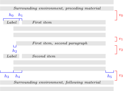
The lengths shown are listed below. The key relationship is that the right edge of the bracket for h1 equals the right edge of the bracket for h4, so that the left edge of the label box is at h3+h4-(h0+h1).
- v0
\topsep+\parskipif the list environment does not start a new paragraph, and\topsep+\parskip+\partopsepif it does- v1
\parsep- v2
\itemsep+\parsep- v3
Same as v0. (This space is affected by whether a blank line appears in the source above the environment; whether a blank line appears in the source below the environment does not matter.)
- h0
\labelwidth- h1
\labelsep- h2
\listparindent- h3
\leftmargin- h4
\itemindent- h5
\rightmargin
The list’s left and right margins, shown above as h3 and h5,
are with respect to the ones provided by the surrounding environment, or
with respect to the page margins for a top-level list. The line width
used for typesetting the list items is \linewidth (see Page layout parameters). For instance, set the list’s left margin to be one
quarter of the distance between the left and right margins of the
enclosing environment with
\setlength{\leftmargin}{0.25\linewidth}.
Page breaking in a list structure is controlled by the three
parameters below. For each, the LaTeX default is
-\@lowpenalty, that is, -51. Because it is negative,
it somewhat encourages a page break at each spot. Change it with,
e.g., \@beginparpenalty=9999; a value of 10000 prohibits a
page break.
\@beginparpenalty¶The page breaking penalty for breaking before the list (default
-51).\@itempenalty¶The page breaking penalty for breaking before a list item (default
-51).\@endparpenalty¶The page breaking penalty for breaking after a list (default
-51).
The package enumitem is useful for customizing lists.
This example has the labels in red. They are numbered, and the left
edge of the label lines up with the left edge of the item text.
See \usecounter.
\usepackage{color}
\newcounter{cnt}
\newcommand{\makeredlabel}[1]{\textcolor{red}{#1.}}
\newenvironment{redlabel}
  {\begin{list}
    {\arabic{cnt}}
    {\usecounter{cnt}
     \setlength{\labelwidth}{0em}
     \setlength{\labelsep}{0.5em}
     \setlength{\leftmargin}{1.5em}
     \setlength{\itemindent}{0.5em} % equals \labelwidth+\labelsep
     \let\makelabel=\makeredlabel
    }
  }
{\end{list}}
8.16.1 \item: An entry in a list
Synopsis:
\item text of item
or
\item[optional-label] text of item
An entry in a list. The entries are prefixed by a label, whose default depends on the list type.
Because the optional label is surrounded by square brackets
‘[...]’, if you have an item whose text starts with [, you
have to hide the bracket inside curly braces, as in: \item
{[} is an open square bracket; otherwise, LaTeX will think it
marks the start of an optional label.
Similarly, if the item does have the optional label and you need a
close square bracket inside that label, you must hide it in the same
way: \item[Close square bracket, {]}]. See LaTeX command syntax.
In this example the enumerate list has two items that use the default label and one that uses the optional label.
\begin{enumerate}
  \item Moe
  \item[sometimes] Shemp
  \item Larry
\end{enumerate}
The first item is labelled ‘1.’, the second item is labelled ‘sometimes’, and the third item is labelled ‘2.’. Because of the optional label in the second item, the third item is not labelled ‘3.’.
8.16.2 trivlist: A restricted form of list
Synopsis:
\begin{trivlist}
  ...
\end{trivlist}
A restricted version of the list environment, in which margins are not
indented and an \item without an optional argument produces no
text. It is most often used in macros, to define an environment where
the \item command is part of the environment’s definition. For
instance, the center environment is defined essentially like
this:
\newenvironment{center}
  {\begin{trivlist}\centering\item\relax}
  {\end{trivlist}}
Using trivlist in this way allows the macro to inherit some
common code: combining vertical space of two adjacent environments;
detecting whether the text following the environment should be
considered a new paragraph or a continuation of the previous one;
adjusting the left and right margins for possible nested list
environments.
Specifically, trivlist uses the current values of the list
parameters (see list), except that \parsep is set to the
value of \parskip, and \leftmargin, \labelwidth,
and \itemindent are set to zero.
This example outputs the items as two paragraphs, except that (by default) they have no paragraph indent and are vertically separated.
\begin{trivlist}
\item The \textit{Surprise} is not old; no one would call her old.
\item She has a bluff bow, lovely lines.
\end{trivlist}
8.17 math
Synopsis:
\begin{math}
math
\end{math}
The math environment inserts given math material within
the running text. \(...\) and $...$ are synonyms.
See Math formulas.
8.18 minipage
Synopses:
\begin{minipage}{width}
  contents
\end{minipage}
or
\begin{minipage}[position][height][inner-pos]{width}
  contents
\end{minipage}
Put contents into a box that is width wide. This is like a
small version of a page; it can contain its own footnotes, itemized
lists, etc. (There are some restrictions, including that it cannot have
floats.) This box will not be broken across pages. So minipage
is similar to \parbox (see \parbox) but here you can have
paragraphs.
This example will be 3 inches wide, and has two paragraphs.
\begin{minipage}{3in}
  Stephen Kleene was a founder of the Theory of Computation.

  He was a student of Church, wrote three influential texts,
  was President of the Association for Symbolic Logic,
  and won the National Medal of Science.
\end{minipage}
See below for a discussion of the paragraph indent inside a
minipage.
The required argument width is a rigid length (see Lengths). It gives the width of the box into which contents are typeset.
There are three optional arguments, position, height, and
inner-pos. You need not include all three. For example, get the
default position and set the height with
\begin{minipage}[c][2.54cm]{\columnwidth} contents
\end{minipage}
. (Get the natural height with an empty argument,
[].)
The optional argument position governs how the minipage
vertically aligns with the surrounding material.
c(synonym
m) Default. Positions theminipageso its vertical center lines up with the center of the adjacent text line.t¶Align the baseline of the top line in the
minipagewith the baseline of the surrounding text (plain TeX’s\vtop).b¶Align the baseline of the bottom line in the
minipagewith the baseline of the surrounding text (plain TeX’s\vbox).
To see the effects of these, contrast running this
---\begin{minipage}[c]{0.25in}
  first\\ second\\ third
\end{minipage}
with the results of changing c to b or t.
The optional argument height is a rigid length (see Lengths).
It sets the height of the minipage. You can enter any value
larger than, or equal to, or smaller than the minipage’s natural
height and LaTeX will not give an error or warning. You can also set
it to a height of zero or a negative value.
The final optional argument inner-pos controls the placement of contents inside the box. These are the possible values are (the default is the value of position).
tPlace contents at the top of the box.
cPlace it in the vertical center.
bPlace it at the box bottom.
sStretch contents out vertically; it must contain vertically stretchable space.
The inner-pos argument makes sense when the height option
is set to a value larger than the minipage’s natural height. To
see the effect of the options, run this example with the various choices
in place of b.
Text before
\begin{center}
  ---\begin{minipage}[c][3in][b]{0.25\textwidth}
       first\\ second\\ third
  \end{minipage}
\end{center}
Text after
By default paragraphs are not indented in a minipage. Change
that with a command such as \setlength{\parindent}{1pc} at
the start of contents.
Footnotes in a minipage environment are handled in a way that is
particularly useful for putting footnotes in figures or tables. A
\footnote or \footnotetext command puts the footnote at
the bottom of the minipage instead of at the bottom of the page, and it
uses the \mpfootnote counter instead of the ordinary
footnote counter (see Counters).
This puts the footnote at the bottom of the table, not the bottom of the page.
\begin{center}           % center the minipage on the line
\begin{minipage}{2.5in}
  \begin{center}         % center the table inside the minipage
    \begin{tabular}{ll}
      \textsc{Monarch}  &\textsc{Reign}             \\ \hline
      Elizabeth II      &63 years\footnote{to date} \\
      Victoria          &63 years                   \\
      George III        &59 years
    \end{tabular}
  \end{center}
\end{minipage}
\end{center}
If you nest minipages then there is an oddness when using footnotes.
Footnotes appear at the bottom of the text ended by the next
\end{minipage} which may not be their logical place.
This puts a table containing data side by side with a map graphic. They are vertically centered.
% siunitx to have the S column specifier,
% which aligns numbers on their decimal point.
\usepackage{siunitx}
\newcommand*{\vcenteredhbox}[1]{\begin{tabular}{@{}c@{}}#1\end{tabular}}
  ...
\begin{center}
  \vcenteredhbox{\includegraphics[width=0.3\textwidth]{nyc.png}}
  \hspace{0.1\textwidth}
  \begin{minipage}{0.5\textwidth}
    \begin{tabular}{r|S}
      % \multicolumn to remove vertical bar between column headers
      \multicolumn{1}{r}{Borough} &
      % braces to prevent siunitx from misinterpreting the
      % period as a decimal separator
      {Pop. (million)}  \\ \hline
      The Bronx      &1.5  \\
      Brooklyn       &2.6  \\
      Manhattan      &1.6  \\
      Queens         &2.3  \\
      Staten Island  &0.5
    \end{tabular}
  \end{minipage}
\end{center}
8.19 picture
Synopses:
\begin{picture}(width,height)
   picture command
\end{picture}
or
\begin{picture}(width,height)(xoffset,yoffset)
  picture command
\end{picture}
Where there may be any number of picture command’s.
An environment to create simple pictures containing lines, arrows, boxes, circles, and text. This environment is not obsolete, but new documents typically use much more powerful graphics creation systems, such as TikZ, PSTricks, MetaPost, or Asymptote. None of these are covered in this document; see CTAN.
To start, here’s an example showing the parallelogram law for adding vectors.
\setlength{\unitlength}{1cm}
\begin{picture}(6,6)      % picture box will be 6cm wide by 6cm tall
  \put(0,0){\vector(2,1){4}}  % for every 2 over this vector goes 1 up
    \put(2,1){\makebox(0,0)[l]{\ first leg}}
  \put(4,2){\vector(1,2){2}}
    \put(5,4){\makebox(0,0)[l]{\ second leg}}
  \put(0,0){\vector(1,1){6}}
    \put(3,3){\makebox(0,0)[r]{sum\ }}
\end{picture}
The picture environment has one required argument, a pair of
positive real numbers (width,height). Multiply these by the
value \unitlength to get the nominal size of the output, i.e.
the space that LaTeX reserves on the output page. This nominal size
need not be how large the picture really is; LaTeX will draw things
from the picture outside the picture’s box.
This environment also has an optional argument
(xoffset,yoffset). It is used to shift the origin. Unlike
most optional arguments, this one is not contained in square brackets.
As with the required argument, it consists of a pair of two real
numbers, but these may also be negative or null. Multiply these
by \unitlength to get the coordinates of the point at the
lower-left corner of the picture.
For example, if \unitlength has been set to 1mm, the
command
\begin{picture}(100,200)(10,20)
produces a box of width 100 millimeters and height 200 millimeters. The picture’s origin is the point (10mm,20mm) and so the lower-left corner is there, and the upper-right corner is at (110mm,220mm). When you first draw a picture you typically omit the optional argument, leaving the origin at the lower-left corner. If you then want to modify your picture by shifting everything, you can just add the appropriate optional argument.
Each picture command tells LaTeX where to put something by
providing its position. A position is a pair such as (2.4,-5)
giving the x- and y-coordinates. A coordinate is a not a length,
it is a real number (it may have a decimal point or a minus sign). It
specifies a length in multiples of the unit length \unitlength,
so if \unitlength has been set to 1cm, then the coordinate
2.54 specifies a length of 2.54 centimeters.
LaTeX’s default for \unitlength is 1pt. It is a rigid
length (see Lengths). Change it with the \setlength command
(see \setlength). Make this change only outside of a picture
environment.
The picture environment supports using standard arithmetic
expressions as well as numbers.
Coordinates are given with respect to an origin, which is by default at
the lower-left corner of the picture. Note that when a position appears
as an argument, as with \put(1,2){...}, it is not enclosed in
braces since the parentheses serve to delimit the argument. Also,
unlike in some computer graphics systems, larger y-coordinates are
further up the page, for example, y = 1 is above y = 0.
There are four ways to put things in a picture: \put,
\multiput, \qbezier, and \graphpaper. The most
often used is \put. This
\put(11.3,-0.3){...}
places the object with its reference point at coordinates
(11.3,-0.3). The reference points for various objects will be
described below.
The \put command creates an LR box (see Modes).
Anything that can go in an \mbox (see \mbox & \makebox) can
go in the text argument of the \put command. The reference point
will be the lower left corner of the box. In this picture
\setlength{\unitlength}{1cm}
...\begin{picture}(1,1)
  \put(0,0){\line(1,0){1}}
  \put(0,0){\line(1,1){1}}
\end{picture}
the three dots are just slightly left of the point of the angle formed
by the two lines. (Also, \line(1,1){1} does not call for a
line of length one; rather the line has a change in the x coordinate of
1.)
The \multiput, qbezier, and graphpaper commands are
described below.
You can also use this environment to place arbitrary material at an exact location. For example:
\usepackage{color,graphicx}  % in preamble
  ...
\begin{center}
\setlength{\unitlength}{\textwidth}
\begin{picture}(1,1)      % leave space, \textwidth wide and tall
  \put(0,0){\includegraphics[width=\textwidth]{desertedisland.jpg}}
  \put(0.25,0.35){\textcolor{red}{X Treasure here}}
\end{picture}
\end{center}
The red X will be precisely a quarter of the \textwidth from
the left margin, and 0.35\textwidth up from the bottom of the
picture. Another example of this usage is to put similar code in the
page header to get repeat material on each of a document’s pages.
\put\multiput\qbezier\graphpaper\line\linethickness\thinlines\thicklines\circle\oval\shortstack\vector\makebox(picture)\framebox(picture)\frame\dashbox
8.19.1 \put
Synopsis:
\put(xcoord,ycoord){content}
Place content at the coordinate (xcoord,ycoord). See
the discussion of coordinates and \unitlength in picture.
The content is processed in LR mode (see Modes) so it cannot
contain line breaks.
This includes the text into the picture.
\put(4.5,2.5){Apply the \textit{unpoke} move}
The reference point, the location (4.5,2.5), is the lower left of the text, at the bottom left of the ‘A’.
8.19.2 \multiput
Synopsis:
\multiput(x,y)(delta_x,delta_y){num-copies}{obj}
Copy obj a total of num-copies times, with an increment of delta_x,delta_y. The obj first appears at position (x,y), then at (x+\delta_x,y+\delta_y), and so on.
This draws a simple grid with every fifth line in bold (see also
\graphpaper).
\begin{picture}(10,10)
  \linethickness{0.05mm}
  \multiput(0,0)(1,0){10}{\line(0,1){10}}
  \multiput(0,0)(0,1){10}{\line(1,0){10}}
  \linethickness{0.5mm}
  \multiput(0,0)(5,0){3}{\line(0,1){10}}
  \multiput(0,0)(0,5){3}{\line(1,0){10}}
\end{picture}
8.19.3 \qbezier
Synopsis:
\qbezier(x1,y1)(x2,y2)(x3,y3)
\qbezier[num](x1,y1)(x2,y2)(x3,y3)
Draw a quadratic Bezier curve whose control points are given by the
three required arguments (x1,y1),
(x2,y2), and (x3,y3). That is,
the curve runs from (x1,y1) to (x3,y3), is quadratic, and is
such that the tangent line at (x1,y1) passes through
(x2,y2), as does the tangent line at (x3,y3).
This draws a curve from the coordinate (1,1) to (1,0).
\qbezier(1,1)(1.25,0.75)(1,0)
The curve’s tangent line at (1,1) contains (1.25,0.75), as does the curve’s tangent line at (1,0).
The optional argument num gives the number of calculated
intermediate points. The default is to draw a smooth curve whose
maximum number of points is \qbeziermax (change this value with
\renewcommand).
This draws a rectangle with a wavy top, using \qbezier for
that curve.
\begin{picture}(8,4)
  \put(0,0){\vector(1,0){8}}  % x axis
  \put(0,0){\vector(0,1){4}}  % y axis
  \put(2,0){\line(0,1){3}}       % left side
  \put(4,0){\line(0,1){3.5}}     % right side
  \qbezier(2,3)(2.5,2.9)(3,3.25)
    \qbezier(3,3.25)(3.5,3.6)(4,3.5)
  \thicklines                 % below here, lines are twice as thick
  \put(2,3){\line(4,1){2}}
  \put(4.5,2.5){\framebox{Trapezoidal Rule}}
\end{picture}
8.19.4 \graphpaper
Synopsis:
\graphpaper(x_init,y_init)(x_dimen,y_dimen)
\graphpaper[spacing](x_init,y_init)(x_dimen,y_dimen)
Draw a coordinate grid. Requires the graphpap package.
The grid’s origin is (x_init,y_init).
Grid lines come every spacing units (the default is 10).
The grid extends x_dimen units to the right and y_dimen units up.
All arguments must be positive integers.
This make a grid with seven vertical lines and eleven horizontal lines.
\usepackage{graphpap}    % in preamble
  ...
\begin{picture}(6,20)    % in document body
  \graphpaper[2](0,0)(12,20)
\end{picture}
The lines are numbered every ten units.
8.19.5 \line
Synopsis:
\line(x_run,y_rise){travel}
Draw a line. It slopes such that it vertically rises y_rise for every horizontal x_run. The travel is the total horizontal change—it is not the length of the vector, it is the change in x. In the special case of vertical lines, where (x_run,y_rise)=(0,1), the travel gives the change in y.
This draws a line starting at coordinates (1,3).
\put(1,3){\line(2,5){4}}
For every over 2, this line will go up 5. Because travel specifies that this goes over 4, it must go up 10. Thus its endpoint is (1,3)+(4,10)=(5,13). In particular, note that travel=4 is not the length of the line, it is the change in x.
The arguments x_run and y_rise are integers that can be
positive, negative, or zero. (If both are 0 then LaTeX treats the
second as 1.) With
\put(x_init,y_init){\line(x_run,y_rise){travel}},
if x_run is negative then the line’s ending point has a first
coordinate that is less than x_init. If y_rise is negative
then the line’s ending point has a second coordinate that is less than
y_init.
If travel is negative then you get LaTeX Error: Bad \line or
\vector argument.
Standard LaTeX can only draw lines with a limited range of slopes
because these lines are made by putting together line segments from
pre-made fonts. The two numbers x_run and y_rise must have
integer values from −6 through 6. Also, they must be
relatively prime, so that (x_run,y_rise) can be (2,1) but not
(4,2) (if you choose the latter then instead of lines you get sequences
of arrowheads; the solution is to switch to the former). To get lines
of arbitrary slope and plenty of other shapes in a system like
picture, see the package pict2e
(https://ctan.org/pkg/pict2e). Another solution
is to use a full-featured graphics system such as TikZ, PSTricks,
MetaPost, or Asymptote.
8.19.6 \linethickness
Synopsis:
\linethickness{dim}
Declares the thickness of subsequent horizontal and vertical lines in a
picture to be dim, which must be a positive length
(see Lengths). It differs from \thinlines and
\thicklines in that it does not affect the thickness of slanted
lines, circles, or ovals (see \oval).
8.19.7 \thinlines
Declaration to set the thickness of subsequent lines, circles, and ovals
in a picture environment to be 0.4pt. This is the default
thickness, so this command is unnecessary unless the thickness has been
changed with either \linethickness or \thicklines.
8.19.8 \thicklines
Declaration to set the thickness of subsequent lines, circles, and ovals
in a picture environment to be 0.8pt. See also
\linethickness and \thinlines. This command is illustrated
in the Trapezoidal Rule example of \qbezier.
8.19.9 \circle
Synopsis:
\circle{diameter}
\circle*{diameter}
Produces a circle with a diameter as close as possible to the specified
one. The * form produces a filled-in circle.
This draws a circle of radius 6, centered at (5,7).
\put(5,7){\circle{6}}
The available radii for \circle are, in points, the even
numbers from 2 to 20, inclusive. For \circle* they are all the
integers from 1 to 15.
8.19.10 \oval
Synopsis:
\oval(width,height)
\oval(width,height)[portion]
Produce a rectangle with rounded corners, hereinafter referred to as an oval. The optional argument portion allows you to produce only half or a quarter of the oval. For half an oval take portion to be one of these.
ttop half
bbottom half
rright half
lleft half
Produce only one quarter of the oval by setting portion to
tr, br, bl, or tl.
This draws the top half of an oval that is 3 wide and 7 tall.
\put(5,7){\oval(3,7)[t]}
The (5,7) is the center of the entire oval, not just the center of the top half.
These shapes are not ellipses. They are rectangles whose corners are
made with quarter circles. These circles have a maximum radius of
20pt (see \circle for the sizes). Thus large ovals are just
frames with a small amount of corner rounding.
8.19.11 \shortstack
Synopsis:
\shortstack[position]{line 1 \\ ... }
Produce a vertical stack of objects.
This labels the y axis by writing the word ‘y’ above the word ‘axis’.
\setlength{\unitlength}{1cm}
\begin{picture}(5,2.5)(-0.75,0)
   \put(0,0){\vector(1,0){4}}   % x axis
   \put(0,0){\vector(0,1){2}}   % y
   \put(-0.2,2){\makebox(0,0)[r]{\shortstack[r]{$y$\\ axis}}}
\end{picture}
For a short stack, the reference point is the lower left of the stack.
In the above example the \makebox (see \mbox & \makebox) puts
the stack flush right in a zero width box so in total the short stack
sits slightly to the left of the y axis.
The valid positions are:
rMake objects flush right
lMake objects flush left
cCenter objects (default)
Separate objects into lines with \\. These stacks are short in
that, unlike in a tabular or array environment, here the
rows are not spaced out to be of even baseline skips. Thus, in
\shortstack{X\\o\\o\\X} the first and last rows are taller than
the middle two, and therefore the baseline skip between the two middle
rows is smaller than that between the third and last row. You can
adjust row heights and depths either by putting in the usual interline
spacing with \shortstack{X\\ \strut o\\o\\X} (see \strut),
or explicitly, via an zero-width box \shortstack{X \\
\rule{0pt}{12pt} o\\o\\X} or by using \\’s optional
argument \shortstack{X\\[2pt] o\\o\\X}.
The \shortstack command is also available outside the
picture environment.
8.19.12 \vector
Synopsis:
\vector(x_run,y_rise){travel}
Draw a line ending in an arrow. The slope of that line is: it vertically rises y_rise for every horizontal x_run. The travel is the total horizontal change—it is not the length of the vector, it is the change in x. In the special case of vertical vectors, if (x_run,y_rise)=(0,1), then travel gives the change in y.
For an example see picture.
For elaboration on x_run and y_rise see \line. As
there, the values of x_run and y_rise are limited. For
\vector you must chooses integers between −4 and 4,
inclusive. Also, the two you choose must be relatively prime. Thus,
\vector(2,1){4} is acceptable but \vector(4,2){4} is
not (if you use the latter then you get a sequence of arrowheads).
8.19.13 \makebox (picture)
Synopsis:
\makebox(rec-width,rec-height){text}
\makebox(rec-width,rec-height)[position]{text}
Make a box to hold text. This command fits with the
picture environment, although you can use it outside of there,
because rec-width and rec-height are numbers specifying
distances in terms of the \unitlength (see picture). This
command is similar to the normal \makebox command (see \mbox & \makebox) except here that you must specify the width and height. This
command is fragile (see \protect).
This makes a box of length 3.5 times \unitlength and height 4
times \unitlength.
\put(1,2){\makebox(3.5,4){...}}
The optional argument position specifies where in the box
the text appears. The default is to center it, both horizontally
and vertically. To place it somewhere else, use a string with one or
two of these letters.
tPuts text the top of the box.
bPut text at the bottom.
lPut text on the left.
rPut text on the right.
8.19.14 \framebox (picture)
Synopsis:
\framebox(rec-width,rec-height){text}
\framebox(rec-width,rec-height)[position]{text}
This is the same as \makebox (picture) except that it puts a frame
around the outside of the box that it creates. The reference point is
the bottom left corner of the frame. This command fits with the
picture environment, although you can use it outside of there,
because lengths are numbers specifying the distance in terms of the
\unitlength (see picture). This command is fragile
(see \protect).
This example creates a frame 2.5 inches by 3 inches and puts the text in the center.
\setlength{\unitlength}{1in}
\framebox(2.5,3){test text}
The required arguments are that the rectangle has overall width rect-width units and height rect-height units.
The optional argument position specifies the position of
text; see \makebox (picture) for the values that it can
take.
The rule has thickness \fboxrule and there is a blank space
\fboxsep between the frame and the contents of the box.
For this command, you must specify the width and height. If
you want to just put a frame around some contents whose dimension is
determined in some other way then either use \fbox (see \fbox & \framebox) or \frame (see \frame).
8.19.15 \frame
Synopsis:
\frame{contents}
Puts a rectangular frame around contents. The reference point
is the bottom left corner of the frame. In contrast to
\framebox (see \framebox (picture)), this command puts no
extra space between the frame and the object. It is fragile
(see \protect).
8.19.16 \dashbox
Synopsis:
\dashbox{dash-len}(rect-width,rect-height){text}
\dashbox{dash-len}(rect-width,rect-height)[position]{text}
Create a dashed rectangle around text. This command fits with the
picture environment, although you can use it outside of there,
because lengths are numbers specifying the distance in terms of the
\unitlength (see picture).
The required arguments are: dashes are dash-len units long, with the same length gap, and the rectangle has overall width rect-width units and height rect-height units.
The optional argument position specifies the position of
text; see \makebox (picture) for the values that it can
take.
This shows that you can use non-integer value for dash-len.
\put(0,0){\dashbox{0.1}(5,0.5){My hovercraft is full of eels.}}
Each dash will be 0.1\unitlength long, the box’s width is
5\unitlength and its height is 0.5\unitlength.
As in that example, a dashed box looks best when rect-width and rect-height are multiples of the dash-len.
8.20 quotation & quote
Synopsis:
\begin{quotation}
  text
\end{quotation}
or
\begin{quote}
  text
\end{quote}
Include a quotation. Both environments indent margins on both sides by
\leftmargin and the text is right-justified.
They differ in how they treat paragraphs. In the quotation
environment, paragraphs are indented by 1.5em and the space
between paragraphs is small, 0pt plus 1pt. In the quote
environment, paragraphs are not indented and there is vertical space
between paragraphs (it is the rubber length \parsep).
\begin{quotation} \small\it
  Four score and seven years ago
  ... shall not perish from the earth.
  \hspace{1em plus 1fill}---Abraham Lincoln
\end{quotation}
8.21 tabbing
Synopsis:
\begin{tabbing}
row1col1 \= row1col2 ...  \\
row2col1 \> row2col2 ...  \\
...
\end{tabbing}
Align text in columns, by setting tab stops and tabbing to them much as
was done on a typewriter. This is less often used than the environments
tabular (see tabular) or array (see array) because
in those the width of each column need not be constant and need not be
known in advance.
This example has a first line where the tab stops are set to explicit
widths, ended by a \kill command (which is described below):
\begin{tabbing}
\hspace{1.2in}\=\hspace{1in}\=\kill
Ship                \>Guns             \>Year    \\
\textit{Sophie}     \>14               \>1800    \\
\textit{Polychrest} \>24               \>1803    \\
\textit{Lively}     \>38               \>1804    \\
\textit{Surprise}   \>28               \>1805    \\
\end{tabbing}
Both the tabbing environment and the more widely-used
tabular environment put text in columns. The most important
distinction is that in tabular the width of columns is
determined automatically by LaTeX, while in tabbing the user
sets the tab stops. Another distinction is that tabular
generates a box, but tabbing can be broken across pages.
Finally, while tabular can be used in any mode, tabbing
can be used only in paragraph mode and it always starts a new paragraph,
without indentation.
Moreover, as shown in the example above, there is no need
to use the starred form of the \hspace command at the beginning
of a tabbed row. The right margin of the tabbing environment is
the end of line, so that the width of the environment is
\linewidth.
The tabbing environment contains a sequence of tabbed
rows. The first tabbed row begins immediately after
\begin{tabbing} and each row ends with \\ or
\kill. The last row may omit the \\ and end with just
\end{tabbing}.
At any point the tabbing environment has a current tab stop
pattern, a sequence of n > 0 tab stops, numbered 0, 1,
etc. These create n corresponding columns. Tab stop 0 is
always the left margin, defined by the enclosing environment. Tab
stop number i is set if it is assigned a horizontal
position on the page. Tab stop number i can only be set if
all the stops 0, …, i-1 have already been set; normally
later stops are to the right of earlier ones.
By default any text typeset in a tabbing environment is typeset
ragged right and left-aligned on the current tab stop. Typesetting is
done in LR mode (see Modes).
The following commands can be used inside a tabbing environment.
They are all fragile (see \protect).
\\ (tabbing)¶End a tabbed line and typeset it.
\= (tabbing)¶Sets a tab stop at the current position.
\> (tabbing)¶-
Advances to the next tab stop.
\<¶Put following text to the left of the local margin (without changing the margin). Can only be used at the start of the line.
\+¶Moves the left margin of the next and all the following commands one tab stop to the right, beginning tabbed line if necessary.
\-¶Moves the left margin of the next and all the following commands one tab stop to the left, beginning tabbed line if necessary.
\' (tabbing)¶Moves everything that you have typed so far in the current column, i.e., everything from the most recent
\>,\<,\',\\, or\killcommand, to the previous column and aligned to the right, flush against the current column’s tab stop.\` (tabbing)¶Allows you to put text flush right against any tab stop, including tab stop 0. However, it can’t move text to the right of the last column because there’s no tab stop there. The
\`command moves all the text that follows it, up to the\\or\end{tabbing}command that ends the line, to the right margin of thetabbingenvironment. There must be no\>or\'command between the\`and the\\or\end{tabbing}command that ends the line.\a (tabbing)¶-
In a
tabbingenvironment, the commands\=,\'and\`do not produce accents as usual (see Accents). Instead, use the commands\a=,\a'and\a`. \kill¶Sets tab stops without producing text. Works just like
\\except that it throws away the current line instead of producing output for it. Any\=,\+or\-commands in that line remain in effect.\poptabs¶-
Restores the tab stop positions saved by the last
\pushtabs. \pushtabs¶Saves all current tab stop positions. Useful for temporarily changing tab stop positions in the middle of a
tabbingenvironment.\tabbingsep¶Distance of the text moved by
\'to left of current tab stop.
This example typesets a Pascal function:
\begin{tabbing}
function \= fact(n : integer) : integer;\\
         \> begin \= \+ \\
               \> if \= n > 1 then \+ \\
                        fact := n * fact(n-1) \- \\
                  else \+ \\
                        fact := 1; \-\- \\
            end;\\
\end{tabbing}
The output looks like this.
function fact(n : integer) : integer;
         begin
               if n > 1 then
                  fact := n * fact(n-1);
               else
                  fact := 1;
         end;
This example is just for illustration of the environment. To actually
typeset computer code in typewriter like this, a verbatim environment
(see verbatim) would normally be best. For pretty-printed code,
there are quite a few packages, including algorithm2e,
fancyvrb, listings, and minted.
8.22 table
Synopsis:
\begin{table}[placement]
  table body
  \caption[loftitle]{title}  % optional
  \label{label}              % also optional
\end{table}
A class of floats (see Floats). They cannot be split across pages and so they are not typeset in sequence with the normal text but instead are floated to a convenient place, such as the top of a following page.
This example table environment contains a tabular
\begin{table}
  \centering\small
  \begin{tabular}{ll}
    \multicolumn{1}{c}{\textit{Author}}
      &\multicolumn{1}{c}{\textit{Piece}}  \\ \hline
    Bach            &Cello Suite Number 1  \\
    Beethoven       &Cello Sonata Number 3 \\
    Brahms          &Cello Sonata Number 1
  \end{tabular}
  \caption{Top cello pieces}
  \label{tab:cello}
\end{table}
but you can put many different kinds of content in a table:
the table body may contain text, LaTeX commands, graphics, etc. It is
typeset in a parbox of width \textwidth.
For the possible values of placement and their effect on the float placement algorithm, see Floats.
The label is optional; it is used for cross references (see Cross references).
The \caption command is also optional. It specifies caption
text title for the table (see \caption). By default it is
numbered. If its optional lottitle is present then that text is
used in the list of tables instead of title (see Table of contents, list of figures, list of tables).
In this example the table and caption will float to the bottom of a page, unless it is pushed to a float page at the end.
\begin{table}[b]
  \centering
  \begin{tabular}{r|p{2in}} \hline
    One &The loneliest number \\
    Two &Can be as sad as one.
         It's the loneliest number since the number one.
  \end{tabular}
  \caption{Cardinal virtues}
  \label{tab:CardinalVirtues}
\end{table}
8.23 tabular
Synopsis:
\begin{tabular}[pos]{cols}
  column 1 entry  &column 2 entry  ...  &column n entry \\
  ...
\end{tabular}
or
\begin{tabular*}{width}[pos]{cols}
  column 1 entry  &column 2 entry  ...  &column n entry \\
  ...
\end{tabular*}
Produce a table, a box consisting of a sequence of horizontal rows. Each row consists of items that are aligned vertically in columns. This illustrates many of the features.
\begin{tabular}{l|l}
  \textit{Player name}  &\textit{Career home runs}  \\
  \hline
  Hank Aaron  &755 \\
  Babe Ruth   &714
\end{tabular}
The output will have two left-aligned columns with a vertical bar
between them. This is specified in tabular’s argument
{l|l}.
Put the entries into different columns by separating them with an
ampersand, &. The end of each row is marked with a double
backslash, \\. Put a horizontal rule below a row, after a double
backslash, with \hline.
After the last row the \\ is optional, unless an \hline
command follows to put a rule below the table.
The required and optional arguments to tabular consist of:
- pos
Optional. Specifies the table’s vertical position. The default is to align the table so its vertical center matches the baseline of the surrounding text. There are two other possible alignments:
taligns the table so its top row matches the baseline of the surrounding text, andbaligns on the bottom row.This only has an effect if there is other text. In the common case of a
tabularalone in acenterenvironment this option makes no difference.- cols
Required. Specifies the formatting of columns. It consists of a sequence of the following specifiers, corresponding to the types of column and intercolumn material.
lA column of left-aligned items.
rA column of right-aligned items.
cA column of centered items.
|A vertical line the full height and depth of the environment.
@{text or space}Insert text or space at this location in every row. The text or space material is typeset in LR mode. This text is fragile (see
\protect).If between two column specifiers there is no @-expression then LaTeX’s
book,article, andreportclasses will put on either side of each column a space of width\tabcolsep, which by default is 6pt. That is, by default adjacent columns are separated by 12pt (so\tabcolsepis misleadingly named since it is only half of the separation between tabular columns). In addition, a space of\tabcolsepalso comes before the first column and after the final column, unless you put a@{...}there.If you override the default and use an @-expression then LaTeX does not insert
\tabcolsepso you must insert any desired space yourself, as in@{\hspace{1em}}.An empty expression
@{}will eliminate the space. In particular, sometimes you want to eliminate the space before the first column or after the last one, as in the example below where the tabular lines need to lie on the left margin.\begin{flushleft} \begin{tabular}{@{}l} ... \end{tabular} \end{flushleft}The next example shows text, a decimal point between the columns, arranged so the numbers in the table are aligned on it.
\begin{tabular}{r@{$.$}l}
  $3$ &$14$  \\
  $9$ &$80665$
\end{tabular}
An
\extracolsep{wd}command in an @-expression causes an extra space of width wd to appear to the left of all subsequent columns, until countermanded by another\extracolsep. Unlike ordinary intercolumn space, this extra space is not suppressed by an @-expression. An\extracolsepcommand can be used only in an @-expression in thecolsargument. Below, LaTeX inserts the right amount of intercolumn space to make the entire table 4 inches wide.\begin{tabular*}{4in}{l@{\extracolsep{\fill}}l} Seven times down, eight times up \ldots &such is life! \end{tabular*}To insert commands that are automatically executed before a given column, load the
arraypackage and use the>{...}specifier.p{wd}Each item in the column is typeset in a parbox of width wd, as if it were the argument of a
\parbox[t]{wd}{...}command.A line break double backslash
\\may not appear in the item, except inside an environment likeminipage,array, ortabular, or inside an explicit\parbox, or in the scope of a\centering,\raggedright, or\raggedleftdeclaration (when used in ap-column element these declarations must appear inside braces, as with{\centering .. \\ ..}). Otherwise LaTeX will misinterpret the double backslash as ending the tabular row. Instead, to get a line break in there use\newline(see\newline).*{num}{cols}Equivalent to num copies of cols, where num is a positive integer and cols is a list of specifiers. Thus the specifier
\begin{tabular}{|*{3}{l|r}|}is equivalent to the specifier\begin{tabular}{|l|rl|rl|r|}. Note that cols may contain another*-expression.
- width
Required for
tabular*, not allowed fortabular. Specifies the width of thetabular*environment. The space between columns should be rubber, as with@{\extracolsep{\fill}}, to allow the table to stretch or shrink to make the specified width, or else you are likely to get theUnderfull \hbox (badness 10000) in alignment ...warning.
Parameters that control formatting:
\arrayrulewidth¶A length that is the thickness of the rule created by
|,\hline, and\vlinein thetabularandarrayenvironments. The default is ‘.4pt’. Change it as in\setlength{\arrayrulewidth}{0.8pt}.\arraystretch¶A factor by which the spacing between rows in the
tabularandarrayenvironments is multiplied. The default is ‘1’, for no scaling. Change it as\renewcommand{\arraystretch}{1.2}.\doublerulesep¶A length that is the distance between the vertical rules produced by the
||specifier. The default is ‘2pt’.\tabcolsep¶A length that is half of the space between columns. The default is ‘6pt’. Change it with
\setlength.
The following commands can be used inside the body of a tabular
environment, the first two inside an entry and the second two between
lines:
8.23.1 \multicolumn
Synopsis:
\multicolumn{numcols}{cols}{text}
Make an array or tabular entry that spans several columns.
The first argument numcols gives the number of columns to span.
The second argument cols specifies the formatting of the entry,
with c for centered, l for flush left, or r for
flush right. The third argument text gives the contents of that
entry.
In this example, in the first row, the second and third columns are spanned by the single heading ‘Name’.
\begin{tabular}{lccl}
  \textit{ID}       &\multicolumn{2}{c}{\textit{Name}} &\textit{Age} \\
  \hline
  978-0-393-03701-2 &O'Brian &Patrick                  &55           \\
    ...
\end{tabular}
What counts as a column is: the column format specifier for the
array or tabular environment is broken into parts, where
each part (except the first) begins with l, c, r,
or p. So from \begin{tabular}{|r|ccp{1.5in}|}
the parts are |r|, c, c,
and p{1.5in}|.
The cols argument overrides the array or tabular
environment’s intercolumn area default adjoining this multicolumn
entry. To affect that area, this argument can contain vertical bars
| indicating the placement of vertical rules, and @{...}
expressions. Thus if cols is ‘|c|’ then this multicolumn
entry will be centered and a vertical rule will come in the intercolumn
area before it and after it. This table details the exact behavior.
\begin{tabular}{|cc|c|c|}
  \multicolumn{1}{r}{w}       % entry one
    &\multicolumn{1}{|r|}{x}  % entry two
    &\multicolumn{1}{|r}{y}   % entry three
    &z                        % entry four
\end{tabular}
Before the first entry the output will not have a vertical rule because
the \multicolumn has the cols specifier ‘r’ with no
initial vertical bar. Between entry one and entry two there will be a
vertical rule; although the first cols does not have an ending
vertical bar, the second cols does have a starting one. Between
entry two and entry three there is a single vertical rule; despite that
the cols in both of the surrounding multicolumn’s call for
a vertical rule, you only get one rule. Between entry three and entry
four there is no vertical rule; the default calls for one but the
cols in the entry three \multicolumn leaves it out, and
that takes precedence. Finally, following entry four there is a
vertical rule because of the default.
The number of spanned columns numcols can be 1. Besides giving
the ability to change the horizontal alignment, this also is useful to
override for one row the tabular definition’s default intercolumn
area specification, including the placement of vertical rules.
In the example below, in the tabular definition the first column
is specified to default to left justified but in the first row the entry
is centered with \multicolumn{1}{c}{\textsc{Period}}.
Also in the first row, the second and third columns are spanned by a
single entry with \multicolumn{2}{c}{\textsc{Span}},
overriding the specification to center those two columns on the page
range en-dash.
\begin{tabular}{l|r@{--}l}
  \multicolumn{1}{c}{\textsc{Period}}
    &\multicolumn{2}{c}{\textsc{Span}} \\ \hline
  Baroque          &1600           &1760         \\
  Classical        &1730           &1820         \\
  Romantic         &1780           &1910         \\
  Impressionistic  &1875           &1925
\end{tabular}
Although the tabular specification by default puts a vertical
rule between the first and second columns, no such vertical rule appears
in the first row here. That’s because there is no vertical bar in the
cols part of the first row’s first \multicolumn command.
8.23.2 \vline
Draw a vertical line in a tabular or array environment
extending the full height and depth of an entry’s row. Can also be
used in an @-expression, although its synonym vertical
bar | is more common. This command is rarely used in the
body of a table; typically a table’s vertical lines are specified in
tabular’s cols argument and overridden as needed with
\multicolumn (see tabular).
The example below illustrates some pitfalls. In the first row’s second
entry the \hfill moves the \vline to the left edge of the
cell. But that is different than putting it halfway between the two
columns, so between the first and second columns there are two vertical
rules, with the one from the {c|cc} specifier coming before the
one produced by the \vline\hfill. In contrast, the first row’s
third entry shows the usual way to put a vertical bar between two
columns. In the second row, the ghi is the widest entry in its
column so in the \vline\hfill the \hfill has no effect and
the vertical line in that entry appears immediately next to the
g, with no whitespace.
\begin{tabular}{c|cc}
  x   &\vline\hfill y   &\multicolumn{1}{|r}{z} \\ % row 1
  abc &def &\vline\hfill ghi                       % row 2
\end{tabular}
8.23.3 \cline
Synopsis:
\cline{i-j}
In an array or tabular environment, draw a horizontal rule
beginning in column i and ending in column j. The
dash, -, must appear in the mandatory argument. To span a single
column use the number twice, as with \cline{2-2}.
This example puts two horizontal lines between the first and second rows, one line in the first column only, and the other spanning the third and fourth columns. The two lines are side-by-side, at the same height.
\begin{tabular}{llrr}
  a &b &c &d \\ \cline{1-1} \cline{3-4}
  e &f &g &h
\end{tabular}
8.23.4 \hline
Draw a horizontal line the width of the enclosing tabular or
array environment. It’s most commonly used to draw a line at the
top, bottom, and between the rows of a table.
In this example the top of the table has two horizontal rules, one above
the other, that span both columns. The bottom of the table has a single
rule spanning both columns. Because of the \hline, the
tabular second row’s line ending double backslash \\
is required.
\begin{tabular}{ll} \hline\hline
  Baseball   &Red Sox  \\
  Basketball &Celtics  \\ \hline
\end{tabular}
8.24 thebibliography
Synopsis:
\begin{thebibliography}{widest-label}
  \bibitem[label]{cite_key}
  ...
\end{thebibliography}
Produce a bibliography or reference list. There are two ways to produce bibliographic lists. This environment is suitable when you have only a few references and can maintain the list by hand. See Using BibTeX, for a more sophisticated approach.
This shows the environment with two entries.
This work is based on \cite{latexdps}.
Together they are \cite{latexdps, texbook}.
  ...
\begin{thebibliography}{9}
\bibitem{latexdps}
  Leslie Lamport.
  \textit{\LaTeX{}: a document preparation system}.
  Addison-Wesley, Reading, Massachusetts, 1993.
\bibitem{texbook}
  Donald Ervin Knuth.
  \textit{The \TeX book}.
  Addison-Wesley, Reading, Massachusetts, 1983.
\end{thebibliography}
This styles the first reference as ‘[1] Leslie ...’, and so that
... based on \cite{latexdps} produces the matching
‘... based on [1]’. The second \cite produces ‘[1,
2]’. You must compile the document twice to resolve these references.
The mandatory argument widest-label is text that, when typeset, is
as wide as the widest item label produced by the \bibitem
commands. The tradition is to use 9 for bibliographies with less
than 10 references, 99 for ones with less than 100, etc.
The bibliographic list is headed by a title such as ‘Bibliography’.
To change it there are two cases. In the book and report
classes, where the top level sectioning is \chapter and the
default title is ‘Bibliography’, that title is in the macro
\bibname. For article, where the class’s top level
sectioning is \section and the default is ‘References’, the
title is in macro \refname. Change it by redefining the command,
as with \renewcommand{\refname}{Cited references}, after
\begin{document}.
Language support packages such as babel will automatically
redefine \refname or \bibname to fit the selected
language.
See list, for the list layout control parameters.
8.24.1 \bibitem
Synopsis:
\bibitem{cite_key}
or
\bibitem[label]{cite_key}
Generate an entry labeled by default by a number generated using the
enumi counter. The citation key
cite_key can be any string of
letters, numbers, and punctuation symbols (but not comma).
See thebibliography, for an example.
When provided, the optional label becomes the entry label and the
enumi counter is not incremented. With this
\begin{thebibliography}
\bibitem[Lamport 1993]{latexdps}
  Leslie Lamport.
  \textit{\LaTeX{}: a document preparation system}.
  Addison-Wesley, Reading, Massachusetts, 1993.
\bibitem{texbook}
  Donald Ervin Knuth.
  \textit{The \TeX book}.
  Addison-Wesley, Reading, Massachusetts, 1983.
\end{thebibliography}
the first entry will be styled as ‘[Lamport 1993] Leslie ...’ (The
amount of horizontal space that LaTeX leaves for the label depends on
the widest-label argument of the thebibliography
environment; see thebibliography.) Similarly, ... based on
\cite{latexdps} will produce ‘... based on [Lamport 1994]’.
If you mix \bibitem entries having a label with those that
do not then LaTeX will number the unlabelled ones sequentially. In
the example above the texbook entry will appear as ‘[1]
Donald ...’, despite that it is the second entry.
If you use the same cite_key twice then you get ‘LaTeX Warning: There were multiply-defined labels’.
Under the hood, LaTeX remembers the cite_key and label
information because \bibitem writes it to the auxiliary file
jobname.aux (see Jobname). For instance, the above
example causes the two \bibcite{latexdps}{Lamport, 1993} and
\bibcite{texbook}{1} to appear in that file. The .aux
file is read by the \begin{document} command and then the
information is available for \cite commands. This explains why
you need to run LaTeX twice to resolve references: once to write it
out and once to read it in.
Because of this two-pass algorithm, when you add a \bibitem or
change its cite_key you may get ‘LaTeX Warning: Label(s) may
have changed. Rerun to get cross-references right’. Fix it by
recompiling.
8.24.2 \cite
Synopsis:
\cite{keys}
or
\cite[subcite]{keys}
Generate as output a citation to the references associated with
keys. The mandatory keys is a citation key, or a
comma-separated list of citation keys (see \bibitem).
This
The ultimate source is \cite{texbook}.
  ...
\begin{thebibliography}
\bibitem{texbook}
  Donald Ervin Knuth.
  \textit{The \TeX book}.
  Addison-Wesley, Reading, Massachusetts, 1983.
\end{thebibliography}
produces output like ‘... source is [1]’. You can change the
appearance of the citation and of the reference by using bibliography
styles if you generate automatically the thebibliography
environment. More information in Using BibTeX.
The optional argument subcite is appended to the citation. For
example, See 14.3 in \cite[p.~314]{texbook} might produce
‘See 14.3 in [1, p. 314]’.
In addition to what appears in the output, \cite writes
information to the auxiliary file jobname.aux
(see Jobname). For instance, \cite{latexdps} writes
‘\citation{latexdps}’ to that file. This information is used by
BibTeX to include in your reference list only those works that you
have actually cited; see \nocite also.
If keys is not in your bibliography information then you get
‘LaTeX Warning: There were undefined references’, and in the output
the citation shows as a boldface question mark between square brackets.
There are two possible causes. If you have mistyped something, as in
\cite{texbok} then you need to correct the spelling. On the
other hand, if you have just added or modified the bibliographic
information and so changed the .aux file (see \bibitem) then
the fix may be to run LaTeX again.
8.24.3 \nocite
Synopsis:
\nocite{keys}
Produces no output but writes keys to the auxiliary file jobname.aux (see Jobname).
The mandatory argument keys is a comma-separated list of one or
more citation keys (see \bibitem). This information is used by
BibTeX to include these works in your reference list even though you
have not explicitly cited them (see \cite).
8.24.4 Using BibTeX
As described in thebibliography (see thebibliography), a
sophisticated approach to managing bibliographies is provided by the
BibTeX program. This is only an introduction; see the full
documentation on CTAN (see CTAN: The Comprehensive TeX Archive Network).
With BibTeX, you don’t use the thebibliography environment
directly (see thebibliography). Instead, include these lines:
\bibliographystyle{bibstyle}
\bibliography{bibfile1, bibfile2, ...}
The bibstyle refers to a file bibstyle.bst, which defines how your citations will look. The standard bibstyle’s distributed with BibTeX are:
alphaLabels are formed from name of author and year of publication. The bibliographic items are sorted alphabetically.
plainLabels are integers. Sort the bibliographic items alphabetically.
unsrtLike
plain, but entries are in order of citation.abbrvLike
plain, but more compact labels.
Many, many other BibTeX style files exist, tailored to the demands of various publications. See the CTAN topic https://ctan.org/topic/bibtex-sty.
The \bibliography command is what actually produces the
bibliography. Its argument is a comma-separated list, referring to
files named bibfile1.bib, bibfile2.bib,
… These contain your database in BibTeX format. This shows a
typical couple of entries in that format.
@book{texbook,
  title     = {The {{\TeX}}book},
  author    = {D.E. Knuth},
  isbn      = {0201134489},
  series    = {Computers \& typesetting},
  year      = {1983},
  publisher = {Addison-Wesley}
}
@book{sexbook,
    author    = {W.H. Masters and V.E. Johnson},
    title     = {Human Sexual Response},
    year      = {1966},
    publisher = {Bantam Books}
}
Only the bibliographic entries referred to via \cite and
\nocite will be listed in the document’s bibliography. Thus you
can keep all your sources together in one file, or a small number of
files, and rely on BibTeX to include in this document only those that
you used.
With BibTeX, the keys argument to \nocite can also be
the single character ‘*’. This means to implicitly cite all
entries from all given bibliographies.
8.24.4.1 BibTeX error messages
If you forget to use \bibliography or \bibliographystyle
in your document (or, less likely, any \cite or \nocite
command), BibTeX will issue an error message. Because BibTeX
can be used with any program, not just LaTeX, the error messages
refer to the internal commands read by BibTeX (from the .aux
file), rather than the user-level commands described above.
Here is a table showing internal commands mentioned in the BibTeX errors, and the corresponding user-level commands.
For example, if your document has no \bibliographystyle
command, BibTeX complains as follows:
I found no \bibstyle command---while reading file document.aux
8.25 theorem
Synopsis:
\begin{theorem}
  theorem body
\end{theorem}
Produces ‘Theorem n’ in boldface followed by theorem
body in italics. The numbering possibilities for n are described under
\newtheorem (see \newtheorem).
\newtheorem{lem}{Lemma}      % in preamble
\newtheorem{thm}{Theorem}
  ...
\begin{lem}                  % in  document body
  text of lemma
\end{lem}

The next result follows immediately.
\begin{thm}[Gauss]   %  put `Gauss' in parens after theorem head
  text of theorem
\end{thm}
Most new documents use the packages amsthm and amsmath
from the American Mathematical Society. Among other things these
packages include a large number of options for theorem environments,
such as styling options.
8.26 titlepage
Synopsis:
\begin{titlepage}
  ... text and spacing ...
\end{titlepage}
Create a title page, a page with no printed page number or heading and with succeeding pages numbered starting with page one.
In this example all formatting, including vertical spacing, is left to the author.
\begin{titlepage}
\vspace*{\stretch{1}}
\begin{center}
{\huge\bfseries Thesis \\[1ex]
title} \\[6.5ex]
{\large\bfseries Author name} \\
\vspace{4ex}
Thesis submitted to \\[5pt]
\textit{University name} \\[2cm]
in partial fulfilment for the award of the degree of \\[2cm]
\textsc{\Large Doctor of Philosophy} \\[2ex]
\textsc{\large Mathematics} \\[12ex]
\vfill
Department of Mathematics \\
Address \\
\vfill
\today
\end{center}
\vspace{\stretch{2}}
\end{titlepage}
To instead produce a standard title page without a titlepage
environment, use \maketitle (see \maketitle).
8.27 verbatim
Synopsis:
\begin{verbatim}
literal-text
\end{verbatim}
A paragraph-making environment in which LaTeX produces as output
exactly what you type as input. For instance inside literal-text
the backslash \ character does not start commands, it
produces a printed ‘\’, and carriage returns and blanks are taken
literally. The output appears in a monospaced typewriter-like font
(\tt).
\begin{verbatim}
Symbol swearing: %&$#?!.
\end{verbatim}
The only restriction on literal-text is that it cannot include
the string \end{verbatim}.
You cannot use the verbatim environment in the argument to macros, for
instance in the argument to a \section. This is not the same as
commands being fragile (see \protect), instead it just cannot work,
as the verbatim environment changes the catcode regime before
processing its contents, and restore it immediately afterward,
nevertheless with a macro argument the content of the argument has
already be converted to a token list along the catcode regime in effect
when the macro was called. However, the cprotect package can
help with this.
One common use of verbatim input is to typeset computer code. There are
packages that are an improvement the verbatim environment. For
instance, one improvement is to allow the verbatim inclusion of external
files, or parts of those files. Such packages include listings,
and minted.
A package that provides many more options for verbatim environments is
fancyvrb. Another is verbatimbox.
For a list of all the relevant packages, see CTAN (see CTAN: The Comprehensive TeX Archive Network).
8.27.1 \verb
Synopsis:
\verb char literal-text char \verb* char literal-text char
Typeset literal-text as it is input, including special characters
and spaces, using the typewriter (\tt) font.
This example shows two different invocations of \verb.
This is \verb!literally! the biggest pumpkin ever. And this is the best squash, \verb+literally!+
The first \verb has its literal-text surrounded with
exclamation point, !. The second instead uses plus, +,
because the exclamation point is part of literal-text.
The single-character delimiter char surrounds
literal-text—it must be the same character before and after.
No spaces come between \verb or \verb* and char,
or between char and literal-text, or between
literal-text and the second occurrence of char (the
synopsis shows a space only to distinguish one component from the
other). The delimiter must not appear in literal-text. The
literal-text cannot include a line break.
The *-form differs only in that spaces are printed with a visible
space character.
The output from this will include a visible space on both side of word ‘with’:
The command's first argument is \verb*!filename with extension! and ...
For typesetting Internet addresses, urls, the package url
is a better option than the \verb command, since
it allows line breaks.
For computer code there are many packages with advantages over
\verb. One is listings, another is minted.
You cannot use \verb in the argument to a macro, for instance in
the argument to a \section. It is not a question of \verb
being fragile (see \protect), instead it just cannot work, as the
\verb command changes the catcode regime before reading its
argument, and restore it immediately afterward, nevertheless with a
macro argument the content of the argument has already be converted to a
token list along the catcode regime in effect when the macro was called.
However, the cprotect package can help with this.
8.28 verse
Synopsis:
\begin{verse}
line1 \\
line2 \\
...
\end{verse}
An environment for poetry.
Here are two lines from Shakespeare’s Romeo and Juliet.
Then plainly know my heart's dear love is set \\ On the fair daughter of rich Capulet.
Separate the lines of each stanza with \\, and use one or more
blank lines to separate the stanzas.
\begin{verse}
\makebox[\linewidth][c]{\textit{Shut Not Your Doors} ---Walt Whitman}
\\[1\baselineskip]
Shut not your doors to me proud libraries, \\
For that which was lacking on all your well-fill'd shelves, \\
\qquad yet needed most, I bring, \\
Forth from the war emerging, a book I have made, \\
The words of my book nothing, the drift of it every thing, \\
A book separate, not link'd with the rest nor felt by the intellect, \\
But you ye untold latencies will thrill to every page.
\end{verse}
The output has margins indented on the left and the right, paragraphs are not indented, and the text is not right-justified.
9 Line breaking
The first thing LaTeX does when processing ordinary text is to translate your input file into a sequence of glyphs and spaces. To produce a printed document, this sequence must be broken into lines (and these lines must be broken into pages).
LaTeX usually does the line (and page) breaking in the text body for you but in some environments you manually force line breaks.
A common workflow is to get a final version of the document content before taking a final pass through and considering line breaks (and page breaks). This differs from word processing, where you are formatting text as you input it. Putting these off until the end prevents a lot of fiddling with breaks that will change anyway.
\\\obeycr&\restorecr\newline\-(discretionary hyphen)\discretionary(generalized hyphenation point)\fussy&\sloppy\hyphenation\linebreak&\nolinebreak
9.1 \\
Synopsis, one of:
\\ \\[morespace]
or one of:
\\* \\*[morespace]
End the current line. The optional argument morespace specifies
extra vertical space to be inserted before the next line. This is a
rubber length (see Lengths) and can be negative. The text before
the line break is set at its normal length, that is, it is not stretched
to fill out the line width. This command is fragile (see \protect).
\title{My story: \\[0.25in]
a tale of woe}
The starred form, \\*, tells LaTeX not to start a new page
between the two lines, by issuing a \nobreak.
Explicit line breaks in the main text body are unusual in LaTeX. In
particular, don’t start new paragraphs with \\. Instead leave a
blank line between the two paragraphs. And don’t put in a sequence of
\\’s to make vertical space. Instead use
\vspace{length}, or
\leavevmode\vspace{length}, or
\vspace*{length} if you want the space to not be thrown
out at the top of a new page (see \vspace).
The \\ command is mostly used outside of the main flow of text
such as in a tabular or array environment or in an
equation environment.
The \\ command is a synonym for \newline
(see \newline) under ordinary circumstances (an example of an
exception is the p{...} column in a tabular
environment; see tabular).
The \\ command is a macro, and its definition changes by context
so that its definition in normal text, a center environment, a
flushleft environment, and a tabular are all different.
In normal text when it forces a linebreak it is essentially a shorthand
for \newline. It does not end horizontal mode or end the
paragraph, it just inserts some glue and penalties so that when the
paragraph does end a linebreak will occur at that point, with the short
line padded with white space.
You get ‘LaTeX Error: There's no line here to end’ if you use
\\ to ask for a new line, rather than to end the current line.
An example is if you have \begin{document}\\ or, more likely,
something like this.
\begin{center}
\begin{minipage}{0.5\textwidth}
\\
In that vertical space put your mark.
\end{minipage}
\end{center}
Fix it by replacing the double backslash with something like
\vspace{\baselineskip}.
9.2 \obeycr & \restorecr
The \obeycr command makes a return in the input file (‘^^M’,
internally) the same as \\, followed by \relax. So each
new line in the input will also be a new line in the output. The
\restorecr command restores normal line-breaking behavior.
This is not the way to show verbatim text or computer code. Use
verbatim (see verbatim) instead.
With LaTeX’s usual defaults, this
aaa bbb \obeycr ccc ddd eee \restorecr fff ggg hhh iii
produces output like this.
aaa bbb ccc ddd eee fff ggg hhh iii
The indents are paragraph indents.
9.3 \newline
In ordinary text, this ends a line in a way that does not right-justify
it, so the text before the end of line is not stretched. That is, in
paragraph mode (see Modes), the \newline command is
equivalent to double-backslash (see \\). This command is fragile
(see \protect).
However, the two commands are different inside a tabular or
array environment. In a column with a specifier producing a
paragraph box such as typically p{...}, \newline will
insert a line end inside of the column; that is, it does not break the
entire tabular row. To break the entire row use \\ or its
equivalent \tabularnewline.
This will print ‘Name:’ and ‘Address:’ as two lines in a single cell of the table.
\begin{tabular}{p{1in}@{\hspace{2in}}p{1in}}
Name: \newline Address: &Date: \\ \hline
\end{tabular}
The ‘Date:’ will be baseline-aligned with ‘Name:’.
9.4 \- (discretionary hyphen)
Tell LaTeX that it may hyphenate the word at that point. When you
insert \- commands in a word, the word will only be hyphenated at
those points and not at any of the other hyphenation points that
LaTeX might otherwise have chosen. This command is robust
(see \protect).
LaTeX is good at hyphenating and usually finds most of the correct
hyphenation points, while almost never using an incorrect one. The
\- command is for exceptional cases.
For example, LaTeX does not ordinarily hyphenate words containing a hyphen. Below, the long and hyphenated word means LaTeX has to put in unacceptably large spaces to set the narrow column.
\begin{tabular}{rp{1.75in}}
Isaac Asimov &The strain of
anti-intellectualism
% an\-ti-in\-tel\-lec\-tu\-al\-ism
has been a constant thread winding its way through our
political and cultural life, nurtured by
the false notion that democracy means that
`my ignorance is just as good as your knowledge'.
\end{tabular}
Commenting out the third line and uncommenting the fourth makes a much better fit.
The \- command only allows LaTeX to break there, it does not
require that it break there. You can force a split with something
like Hef-\linebreak feron. Of course, if you later change the
text then this forced break may look out of place, so this approach
requires care.
9.5 \discretionary (generalized hyphenation point)
Synopsis:
\discretionary{pre-break}{post-break}{no-break}
Handle word changes around hyphens. This command is not often used in LaTeX documents.
If a line break occurs at the point where \discretionary appears
then TeX puts pre-break at the end of the current line and puts
post-break at the start of the next line. If there is no line
break here then TeX puts no-break.
In ‘difficult’ the three letters ffi form a ligature. But
TeX can nonetheless break between the two ‘f’’s with this.
di\discretionary{f-}{fi}{ffi}cult
Note that users do not have to do this. It is typically handled automatically by TeX’s hyphenation algorithm.
9.6 \fussy & \sloppy
Declarations to make TeX more picky or less picky about line
breaking. Declaring \fussy usually avoids too much space between
words, at the cost of an occasional overfull box. Conversely,
\sloppy avoids overfull boxes while suffering loose interword
spacing.
The default is \fussy. Line breaking in a paragraph is
controlled by whichever declaration is current at the end of the
paragraph, i.e., at the blank line or \par or displayed
equation ending that paragraph. So to affect the line breaks, include
that paragraph-ending material in the scope of the command.
9.6.1 sloppypar
Synopsis:
\begin{sloppypar}
... paragraphs ...
\end{sloppypar}
Typeset the paragraphs with \sloppy in effect (see \fussy & \sloppy). Use this to locally adjust line breaking, to avoid
‘Overfull box’ or ‘Underfull box’ errors.
The example is simple.
\begin{sloppypar}
Her plan for the morning thus settled, she sat quietly down to her
book after breakfast, resolving to remain in the same place and the
same employment till the clock struck one; and from habitude very
little incommoded by the remarks and ejaculations of Mrs.\ Allen,
whose vacancy of mind and incapacity for thinking were such, that
as she never talked a great deal, so she could never be entirely
silent; and, therefore, while she sat at her work, if she lost her
needle or broke her thread, if she heard a carriage in the street,
or saw a speck upon her gown, she must observe it aloud, whether
there were anyone at leisure to answer her or not.
\end{sloppypar}
9.7 \hyphenation
Synopsis:
\hyphenation{word1 ...}
Declares allowed hyphenation points within the words in the list. The
words in that list are separated by spaces. Show permitted points for
hyphenation with a dash character, -.
Here is an example:
\hyphenation{hat-er il-lit-e-ra-ti tru-th-i-ness}
Use lowercase letters. TeX will only hyphenate if the word matches
exactly, no inflections are tried. Multiple \hyphenation
commands accumulate.
9.8 \linebreak & \nolinebreak
Synopses, one of:
\linebreak \linebreak[zero-to-four]
or one of these.
\nolinebreak \nolinebreak[zero-to-four]
Encourage or discourage a line break. The optional zero-to-four
is an integer lying between 0 and 4 that allows you to soften the
instruction. The default is 4, so that without the optional argument
these commands entirely force or prevent the break. But for instance,
\nolinebreak[1] is a suggestion that another place may be better.
The higher the number, the more insistent the request. Both commands
are fragile (see \protect).
Here we tell LaTeX that a good place to put a linebreak is after the standard legal text.
\boilerplatelegal{} \linebreak[2]
We especially encourage applications from members of traditionally
underrepresented groups.
When you issue \linebreak, the spaces in the line are stretched
out so that the break point reaches the right margin. See \\
and \newline, to have the spaces not stretched out.
10 Page breaking
Ordinarily LaTeX automatically takes care of breaking output into pages with its usual aplomb. But if you are writing commands, or tweaking the final version of a document, then you may need to understand how to influence its actions.
LaTeX’s algorithm for splitting a document into pages is more complex than just waiting until there is enough material to fill a page and outputting the result. Instead, LaTeX typesets more material than would fit on the page and then chooses a break that is optimal in some way (it has the smallest badness). An example of the advantage of this approach is that if the page has some vertical space that can be stretched or shrunk, such as with rubber lengths between paragraphs, then LaTeX can use that to avoid widow lines (where a new page starts with the last line of a paragraph; LaTeX can squeeze the extra line onto the first page) and orphans (where the first line of paragraph is at the end of a page; LaTeX can stretch the material of the first page so the extra line falls on the second page). Another example is where LaTeX uses available vertical shrinkage to fit on a page not just the header for a new section but also the first two lines of that section.
But LaTeX does not optimize over the entire document’s set of page breaks. So it can happen that the first page break is great but the second one is lousy; to break the current page LaTeX doesn’t look as far ahead as the next page break. So occasionally you may want to influence page breaks while preparing a final version of a document.
See Layout, for more material that is relevant to page breaking.
10.1 \clearpage & \cleardoublepage
Synopsis:
\clearpage
or
\cleardoublepage
End the current page and output all of the pending floating figures and
tables (see Floats). If there are too many floats to fit on the
page then LaTeX will put in extra pages containing only floats. In
two-sided printing, \cleardoublepage also makes the next page of
content a right-hand page, an odd-numbered page, if necessary inserting
a blank page. The \clearpage command is robust while
\cleardoublepage is fragile (see \protect).
LaTeX’s page breaks are optimized so ordinarily you only use this command in a document body to polish the final version, or inside commands.
The \cleardoublepage command will put in a blank page, but it
will have the running headers and footers. To get a really blank
page, use this command.
\let\origdoublepage\cleardoublepage
\newcommand{\clearemptydoublepage}{%
\clearpage
{\pagestyle{empty}\origdoublepage}%
}
If you want LaTeX’s standard \chapter command to do this then
add the line \let\cleardoublepage\clearemptydoublepage. (Of
course this affects all uses of \cleardoublepage, not just the
one in \chapter.)
The command \newpage (see \newpage) also ends the current
page, but without clearing pending floats. And, if LaTeX is in
two-column mode then \newpage ends the current column while
\clearpage and \cleardoublepage end the current page.
10.2 \newpage
Synopsis:
\newpage
End the current page. This command is robust (see \protect).
LaTeX’s page breaks are optimized so ordinarily you only use this command in a document body to polish the final version, or inside commands.
While the commands \clearpage and \cleardoublepage also
end the current page, in addition they clear pending floats
(see \clearpage & \cleardoublepage). And, if LaTeX is in
two-column mode then \clearpage and \cleardoublepage end
the current page, possibly leaving an empty column, while
\newpage only ends the current column.
In contrast with \pagebreak (see \pagebreak & \nopagebreak),
the \newpage command will cause the new page to start right where
requested. This
Four score and seven years ago our fathers brought forth on this continent, \newpage \noindent a new nation, conceived in Liberty, and dedicated to the proposition that all men are created equal.
makes a new page start after ‘continent’, and the cut-off line is
not right justified. In addition, \newpage does not vertically
stretch out the page, as \pagebreak does.
10.3 \enlargethispage
Synopsis, one of:
\enlargethispage{size}
\enlargethispage*{size}
Enlarge the \textheight for the current page. The required
argument size must be a rigid length (see Lengths). It may be
positive or negative. This command is fragile (see \protect).
A common strategy is to wait until you have the final text of a document, and then pass through it tweaking line and page breaks. This command allows you some page size leeway.
This will allow one extra line on the current page.
\enlargethispage{\baselineskip}
The starred form \enlargesthispage* tries to squeeze the material
together on the page as much as possible, for the common use case of
getting one more line on the page. This is often used together with an
explicit \pagebreak.
10.4 \pagebreak & \nopagebreak
Synopses:
\pagebreak \pagebreak[zero-to-four]
or
\nopagebreak \nopagebreak[zero-to-four]
Encourage or discourage a page break. The optional zero-to-four
is an integer that allows you to soften the request. The default is 4,
so that without the optional argument these commands entirely force or
prevent the break. But for instance \nopagebreak[1] suggests to
LaTeX that another spot might be preferable. The higher the number,
the more insistent the request. Both commands are fragile
(see \protect).
LaTeX’s page endings are optimized so ordinarily you only use these commands in a document body to polish the final version, or inside commands.
If you use these inside a paragraph, they apply to the point following the line in which they appear. So this
Four score and seven years ago our fathers brought forth on this continent, \pagebreak a new nation, conceived in Liberty, and dedicated to the proposition that all men are created equal.
does not give a page break at ‘continent’, but instead at
‘nation’, since that is where LaTeX breaks that line. In
addition, with \pagebreak the vertical space on the page is
stretched out where possible so that it extends to the normal bottom
margin. This can look strange, and if \flushbottom is in effect
this can cause you to get ‘Underfull \vbox (badness 10000) has
occurred while \output is active’. See \newpage, for a command that
does not have these effects.
(There is an obsolete declaration \samepage, which tries to only
allow a break between two paragraphs. There is a related environment
samepage, also obsolete. Neither of these work reliably. For
more on keeping material on the same page, see the FAQ entry
https://texfaq.org/FAQ-nopagebrk.)
11 Footnotes
Place a footnote at the bottom of the current page, as here.
Noël Coward quipped that having to read a footnote is like having
to go downstairs to answer the door, while in the midst of making
love.\footnote{%
I wouldn't know, I don't read footnotes.}
You can put multiple footnotes on a page. If the footnote text becomes too long then it will flow to the next page.
You can also produce footnotes by combining the \footnotemark and
the \footnotetext commands, which is useful in special
circumstances.
To make bibliographic references come out as footnotes you need to include a bibliographic style with that behavior (see Using BibTeX).
\footnote\footnotemark\footnotetext- Footnotes in section headings
- Footnotes in a table
- Footnotes of footnotes
11.1 \footnote
Synopsis, one of:
\footnote{text}
\footnote[number]{text}
Place a footnote text at the bottom of the current page.
There are over a thousand footnotes in Gibbon's
\textit{Decline and Fall of the Roman Empire}.\footnote{%
After reading an early version with endnotes David Hume complained,
``One is also plagued with his Notes, according to the present Method
of printing the Book'' and suggested that they ``only to be printed
at the Margin or the Bottom of the Page.''}
The optional argument number allows you to specify the number of
the footnote. If you use this then LaTeX does not increment the
footnote counter.
By default, LaTeX uses arabic numbers as footnote markers. Change
this with something like
\renewcommand{\thefootnote}{\fnsymbol{footnote}}, which
uses a sequence of symbols (see \alph \Alph \arabic \roman \Roman \fnsymbol: Printing counters). To make this change global put that in the preamble. If
you make the change local then you may want to reset the counter with
\setcounter{footnote}{0}.
LaTeX determines the spacing of footnotes with two parameters.
\footnoterule¶Produces the rule separating the main text on a page from the page’s footnotes. Default dimensions in the standard document classes (except
slides, where it does not appear) is: vertical thickness of0.4pt, and horizontal size of0.4\columnwidthlong. Change the rule with something like this.\renewcommand{\footnoterule}{% Kerns avoid vertical space \kern -3pt % This -3 is negative \hrule width \textwidth height 1pt % of the sum of this 1 \kern 2pt} % and this 2\footnotesep¶-
The height of the strut placed at the beginning of the footnote (see
\strut). By default, this is set to the normal strut for\footnotesizefonts (see Font sizes), therefore there is no extra space between footnotes. This is ‘6.65pt’ for ‘10pt’, ‘7.7pt’ for ‘11pt’, and ‘8.4pt’ for ‘12pt’. Change it as with\setlength{\footnotesep}{11pt}.
The \footnote command is fragile (see \protect).
LaTeX’s default puts many restrictions on where you can use a
\footnote; for instance, you cannot use it in an argument to a
sectioning command such as \chapter (it can only be used in outer
paragraph mode; see Modes). There are some workarounds; see
following sections.
In a minipage environment the \footnote command uses the
mpfootnote counter instead of the footnote counter, so
they are numbered independently. They are shown at the bottom of the
environment, not at the bottom of the page. And by default they are
shown alphabetically. See minipage and Footnotes in a table.
11.2 \footnotemark
Synopsis, one of:
\footnotemark \footnotemark[number]
Put the current footnote mark in the text. To specify associated text
for the footnote see \footnotetext. The optional argument
number causes the command to use that number to determine the
footnote mark. This command can be used in inner paragraph mode
(see Modes).
If you use \footnotemark without the optional argument then it
increments the footnote counter, but if you use the optional
number then it does not. The next example produces several
consecutive footnote markers referring to the same footnote.
The first theorem\footnote{Due to Gauss.}
and the second theorem\footnotemark[\value{footnote}]
and the third theorem.\footnotemark[\value{footnote}]
If there are intervening footnotes then you must remember the value of
the number of the common mark. This example gives the same
institutional affiliation to both the first and third authors
(\thanks is a version of \footnote), by-hand giving the
number of the footnote.
\title{A Treatise on the Binomial Theorem}
\author{J Moriarty\thanks{University of Leeds}
\and A C Doyle\thanks{Durham University}
\and S Holmes\footnotemark[1]}
\begin{document}
\maketitle
This uses a counter to remember the footnote number. The third sentence is followed by the same footnote marker as the first.
\newcounter{footnoteValueSaver}
All babies are illogical.\footnote{%
Lewis Carroll.}\setcounter{footnoteValueSaver}{\value{footnote}}
Nobody is despised who can manage a crocodile.\footnote{%
Captain Hook.}
Illogical persons are despised.\footnotemark[\value{footnoteValueSaver}]
Therefore, anyone who can manage a crocodile is not a baby.
This example accomplishes the same by using the package cleveref.
\usepackage{cleveref}[2012/02/15] % in preamble
\crefformat{footnote}{#2\footnotemark[#1]#3}
...
The theorem is from Evers.\footnote{\label{fn:TE}Tinker, Evers, 1994.}
The corollary is from Chance.\footnote{Evers, Chance, 1990.}
But the key lemma is from Tinker.\cref{fn:TE}
It will work with the package hyperref.
11.3 \footnotetext
Synopsis, one of:
\footnotetext{text}
\footnotetext[number]{text}
Place text at the bottom of the page as a footnote. It pairs with
\footnotemark (see \footnotemark) and can come anywhere after
that command, but must appear in outer paragraph mode (see Modes).
The optional argument number changes the number of the footnote
mark.
See \footnotemark and Footnotes in a table, for usage
examples.
11.4 Footnotes in section headings
Putting a footnote in a section heading, as in:
\section{Full sets\protect\footnote{This material due to ...}}
causes the footnote to appear at the bottom of the page where the
section starts, as usual, but also at the bottom of the table of
contents, where it is not likely to be desired. The simplest way
to have it not appear on the table of contents is to use the optional
argument to \section
\section[Please]{Please\footnote{%
Don't footnote in chapter and section headers!}}
No \protect is needed in front of \footnote here because
what gets moved to the table of contents is the optional argument.
11.5 Footnotes in a table
Inside a tabular or array environment the \footnote
command does not work; there is a footnote mark in the table cell but
the footnote text does not appear. The solution is to use a
minipage environment as here (see minipage).
\begin{center}
\begin{minipage}{\textwidth} \centering
\begin{tabular}{l|l}
\textsc{Ship} &\textsc{Book} \\ \hline
\textit{HMS Sophie} &Master and Commander \\
\textit{HMS Polychrest} &Post Captain \\
\textit{HMS Lively} &Post Captain \\
\textit{HMS Surprise} &A number of books\footnote{%
Starting with \textit{HMS Surprise}.}
\end{tabular}
\end{minipage}
\end{center}
Inside a minipage, footnote marks are lowercase letters. Change
that with something like
\renewcommand{\thempfootnote}{\arabic{mpfootnote}}
(see \alph \Alph \arabic \roman \Roman \fnsymbol: Printing counters).
The footnotes in the prior example appear at the bottom of the
minipage. To have them appear at the bottom of the main page, as
part of the regular footnote sequence, use the \footnotemark and
\footnotetext pair and make a new counter.
\newcounter{mpFootnoteValueSaver}
\begin{center}
\begin{minipage}{\textwidth}
\setcounter{mpFootnoteValueSaver}{\value{footnote}} \centering
\begin{tabular}{l|l}
\textsc{Woman} &\textsc{Relationship} \\ \hline
Mona &Attached\footnotemark \\
Diana Villiers &Eventual wife \\
Christine Hatherleigh Wood &Fiance\footnotemark
\end{tabular}
\end{minipage}% percent sign keeps footnote text close to minipage
\stepcounter{mpFootnoteValueSaver}%
\footnotetext[\value{mpFootnoteValueSaver}]{%
Little is known other than her death.}%
\stepcounter{mpFootnoteValueSaver}%
\footnotetext[\value{mpFootnoteValueSaver}]{%
Relationship is unresolved in XXI.}
\end{center}
For a floating table environment (see table), use the
tablefootnote package.
\usepackage{tablefootnote} % in preamble
...
\begin{table}
\centering
\begin{tabular}{l|l}
\textsc{Date} &\textsc{Campaign} \\ \hline
1862 &Fort Donelson \\
1863 &Vicksburg \\
1865 &Army of Northern Virginia\tablefootnote{%
Ending the war.}
\end{tabular}
\caption{Forces captured by US Grant}
\end{table}
The footnote appears at the page bottom and is numbered in sequence with other footnotes.
11.6 Footnotes of footnotes
Particularly in the humanities, authors can have multiple classes of
footnotes, including having footnotes of footnotes. The package
bigfoot extends LaTeX’s default footnote mechanism in many
ways, including allow these two, as in this example.
\usepackage{bigfoot} % in preamble
\DeclareNewFootnote{Default}
\DeclareNewFootnote{from}[alph] % create class \footnotefrom{}
...
The third theorem is a partial converse of the
second.\footnotefrom{%
Noted in Wilson.\footnote{Second edition only.}}
12 Definitions
LaTeX has support for making new commands of many different kinds.
\newcommand&\renewcommand\providecommand\makeatletter&\makeatother\@ifstar\newcounter: Allocating a counter\newlength\newsavebox\newenvironment&\renewenvironment\newtheorem\newfont\protect\ignorespaces & \ignorespacesafterend- xspace package
12.1 \newcommand & \renewcommand
Synopses, one of (three regular forms, three starred forms):
\newcommand{\cmd}{defn}
\newcommand{\cmd}[nargs]{defn}
\newcommand{\cmd}[nargs][optargdefault]{defn}
\newcommand*{\cmd}{defn}
\newcommand*{\cmd}[nargs]{defn}
\newcommand*{\cmd}[nargs][optargdefault]{defn}
or all the same possibilities with \renewcommand instead of
\newcommand:
\renewcommand{\cmd}{defn}
\renewcommand{\cmd}[nargs]{defn}
\renewcommand{\cmd}[nargs][optargdefault]{defn}
\renewcommand*{\cmd}{defn}
\renewcommand*{\cmd}[nargs]{defn}
\renewcommand*{\cmd}[nargs][optargdefault]{defn}
Define or redefine a command (see also \DeclareRobustCommand in
Class and package commands).
The starred form of these two forbids the arguments from containing
multiple paragraphs of text (in plain TeX terms: the commands
are not \long). With the default form, arguments can be
multiple paragraphs.
These are the parameters (examples follow):
- cmd
Required;
\cmdis the command name. It must begin with a backslash,\, and must not begin with the four character string\end. For\newcommand, it must not be already defined. For\renewcommand, this name must already be defined.- nargs
Optional; an integer from 0 to 9, specifying the number of arguments that the command takes, including any optional argument. Omitting this argument is the same as specifying 0, meaning that the command has no arguments. If you redefine a command, the new version can have a different number of arguments than the old version.
- optargdefault ¶
-
Optional; if this argument is present then the first argument of
\cmdis optional, with default value optargdefault (which may be the empty string). If optargdefault is not present then\cmddoes not take an optional argument.That is, if
\cmdis called with a following argument in square brackets, as in\cmd[optval]{...}..., then within defn the parameter#1is set to optval. On the other hand, if\cmdis called without following square brackets then within defn the parameter#1is set to optargdefault. In either case, the required arguments start with#2.Omitting
[optargdefault]from the definition is entirely different from giving the square brackets with empty contents, as in[]. The former says the command being defined takes no optional argument, so#1is the first required argument (if nargs ≥ 1); the latter sets the optional argument#1to the empty string as the default, if no optional argument was given in the call.Similarly, omitting
[optval]from a call is also entirely different from giving the square brackets with empty contents. The former sets#1to the value of optval (assuming the command was defined to take an optional argument); the latter sets#1to the empty string, just as with any other value.If a command is not defined to take an optional argument, but is called with an optional argument, the results are unpredictable: there may be a LaTeX error, there may be incorrect typeset output, or both.
- defn ¶
Required; the text to be substituted for every occurrence of
\cmd. The parameters#1,#2, …,#nargsare replaced by the values supplied when the command is called (or by optargdefault in the case of an optional argument not specified in the call, as just explained).
TeX ignores blanks in the source following a control word
(see Control sequence, control word and control symbol), as in ‘\cmd ’. If you want a space
there, one solution is to type {} after the command
(‘\cmd{} ’), and another solution is to use an explicit control
space (‘\cmd\ ’).
A simple example of defining a new command:
\newcommand{\RS}{Robin Smith} results in \RS being
replaced by the longer text. Redefining an existing command is similar:
\renewcommand{\qedsymbol}{{\small QED}}.
If you use \newcommand and the command name has already been
used then you get something like ‘LaTeX Error: Command \fred
already defined. Or name \end... illegal, see p.192 of the manual’.
Similarly, If you use \renewcommand and the command name has
not been defined then you get something like ‘LaTeX Error: \hank
undefined’.
Here the first definition creates a command with no arguments, and the second, a command with one required argument:
\newcommand{\student}{Ms~O'Leary}
\newcommand{\defref}[1]{Definition~\ref{#1}}
Use the first as in I highly recommend \student{} to you. The
second has a variable argument, so that \defref{def:basis} expands to
Definition~\ref{def:basis}, which ultimately expands to
something like ‘Definition~3.14’.
Similarly, but with two required arguments:
\newcommand{\nbym}[2]{$#1 \times #2$} is invoked as
\nbym{2}{k}.
This example has an optional argument.
\newcommand{\salutation}[1][Sir or Madam]{Dear #1:}
Then \salutation gives ‘Dear Sir or Madam:’ while
\salutation[John] gives ‘Dear John:’. And
\salutation[] gives ‘Dear :’.
This example has an optional argument and two required arguments.
\newcommand{\lawyers}[3][company]{#2, #3, and~#1}
I employ \lawyers[Howe]{Dewey}{Cheatem}.
The output is ‘I employ Dewey, Cheatem, and Howe.’. The optional
argument, Howe, is associated with #1, while
Dewey and Cheatem are associated with #2
and #3. Because of the optional argument,
\lawyers{Dewey}{Cheatem} will give the output ‘I
employ Dewey, Cheatem, and company.’.
The braces around defn do not define a group, that is, they do not
delimit the scope of the result of expanding defn. For example,
with \newcommand{\shipname}[1]{\it #1}, in this sentence,
The \shipname{Monitor} met the \shipname{Merrimac}.
the words ‘met the’, and the period, would incorrectly be in
italics. The solution is to put another pair of braces inside the
definition: \newcommand{\shipname}[1]{{\it #1}}.
12.1.1 Control sequence, control word and control symbol
When reading input TeX converts the stream of read characters into a
sequence of tokens. When TeX sees a backslash \, it will
handle the following characters in a special way in order to make a
control sequence token.
The control sequences fall into two categories:
-
control word, when the control sequence is gathered from a
\followed by at least one ASCII letter (A-Zanda-z), followed by at least one non-letter. -
control symbol, when the control sequence is gathered from a
\followed by one non-letter character.
The sequence of characters so found after the \ is also called
the control sequence name.
Blanks after a control word are ignored and do not produce any
whitespace in the output (see \newcommand & \renewcommand and
Backslash-space, \ ).
Just as the \relax command does nothing, the following input
will simply print ‘Hello!’ :
Hel\relax lo!
This is because blanks after \relax, including the newline, are
ignored, and blanks at the beginning of a line are also ignored
(see Leading blanks).
12.2 \providecommand
Synopses, one of:
\providecommand{\cmd}{defn}
\providecommand{\cmd}[nargs]{defn}
\providecommand{\cmd}[nargs][optargdefault]{defn}
\providecommand*{\cmd}{defn}
\providecommand*{\cmd}[nargs]{defn}
\providecommand*{\cmd}[nargs][optargdefault]{defn}
Defines a command, as long as no command of this name already exists.
If no command of this name already exists then this has the same effect
as \newcommand. If a command of this name already exists then
this definition does nothing. This is particularly useful in a file
that may be loaded more than once, such as a style file.
See \newcommand & \renewcommand, for the description of the arguments.
This example
\providecommand{\myaffiliation}{Saint Michael's College}
\providecommand{\myaffiliation}{Lyc\'ee Henri IV}
From \myaffiliation.
outputs ‘From Saint Michael's College.’. Unlike
\newcommand, the repeated use of \providecommand to (try
to) define \myaffiliation does not give an error.
12.3 \makeatletter & \makeatother
Synopsis:
\makeatletter ... definition of commands with @ in their name .. \makeatother
Use this pair when you redefine LaTeX commands that are named with an
at-sign character ‘@’. The \makeatletter
declaration makes the at-sign character have the category code of a
letter, code 11. The \makeatother declaration sets the
category code of the at-sign to code 12, its default value.
As TeX reads characters, it assigns each one a category code, or
catcode. For instance, it assigns the backslash
character ‘\’ the catcode 0. Command names
consist of a category 0 character, ordinarily backslash, followed
by letters, category 11 characters (except that a command name can
also consist of a category 0 character followed by a single
non-letter symbol).
LaTeX’s source code has the convention that some commands use
@ in their name. These commands are mainly intended for package
or class writers. The convention prevents authors who are just using a
package or class from accidentally replacing such a command with one of
their own, because by default the at-sign has catcode 12.
Use the pair \makeatletter and \makeatother inside a
.tex file, typically in the preamble, when you are defining or
redefining commands named with @, by having them surround your
definition. Don’t use these inside .sty or .cls files
since the \usepackage and \documentclass commands already
arrange that the at-sign has the character code of a letter,
catcode 11.
For a comprehensive list of macros with an at-sign in their names see https://ctan.org/pkg/macros2e.
In this example the class file has a command
\thesis@universityname that the user wants to change. These
three lines should go in the preamble, before the
\begin{document}.
\makeatletter
\renewcommand{\thesis@universityname}{Saint Michael's College}
\makeatother
12.4 \@ifstar
Synopsis:
\newcommand{\mycmd}{\@ifstar{\mycmd@star}{\mycmd@nostar}}
\newcommand{\mycmd@nostar}[nostar-num-args]{nostar-body}
\newcommand{\mycmd@star}[star-num-args]{star-body}
Many standard LaTeX environments or commands have a variant with the
same name but ending with a star character *, an asterisk.
Examples are the table and table* environments and the
\section and \section* commands.
When defining environments, following this pattern is straightforward
because \newenvironment and \renewenvironment allow the
environment name to contain a star. So you just have to write
\newenvironment{myenv} or
\newenvironment{myenv*} and continue the definition as
usual. For commands the situation is more complex as the star not being
a letter cannot be part of the command name. As in the synopsis above,
there will be a user-called command, given above as \mycmd, which
peeks ahead to see if it is followed by a star. For instance, LaTeX
does not really have a \section* command; instead, the
\section command peeks ahead. This command does not accept
arguments but instead expands to one of two commands that do accept
arguments. In the synopsis these two are \mycmd@nostar and
\mycmd@star. They could take the same number of arguments or a
different number, or no arguments at all. As always, in a LaTeX
document a command using an at-sign @ in its name must be
enclosed inside a \makeatletter ... \makeatother block
(see \makeatletter & \makeatother).
This example of \@ifstar defines the command \ciel and a
variant \ciel*. Both have one required argument. A call to
\ciel{blue} will return "not starry blue sky" while
\ciel*{night} will return "starry night sky".
\makeatletter
\newcommand*{\ciel@unstarred}[1]{not starry #1 sky}
\newcommand*{\ciel@starred}[1]{starry #1 sky}
\newcommand*{\ciel}{\@ifstar{\ciel@starred}{\ciel@unstarred}}
\makeatother
In the next example, the starred variant takes a different number of
arguments than the unstarred one. With this definition, Agent 007’s
``My name is \agentsecret*{Bond},
\agentsecret{James}{Bond}.'' is equivalent to entering the commands
``My name is \textsc{Bond}, \textit{James} textsc{Bond}.''
\newcommand*{\agentsecret@unstarred}[2]{\textit{#1} \textsc{#2}}
\newcommand*{\agentsecret@starred}[1]{\textsc{#1}}
\newcommand*{\agentsecret}{%
\@ifstar{\agentsecret@starred}{\agentsecret@unstarred}}
After a command name, a star is handled similarly to an optional
argument. (This differs from environment names in which the star is
part of the name itself and as such could be in any position.) Thus,
it is technically possible to put any number of spaces between the
command and the star. Thus \agentsecret*{Bond} and
\agentsecret *{Bond} are equivalent. However, the
standard practice is not to insert any such spaces.
There are two alternative ways to accomplish the work of
\@ifstar. (1) The suffix package allows the
construct \newcommand\mycommand{unstarred-variant}
followed by
\WithSuffix\newcommand\mycommand*{starred-variant}.
(2) LaTeX provides the xparse package, which allows
this code:
\NewDocumentCommand\foo{s}{\IfBooleanTF#1
{starred-variant}%
{unstarred-variant}%
}
12.5 \newcounter: Allocating a counter
Synopsis, one of:
\newcounter{countername}
\newcounter{countername}[supercounter]
Globally defines a new counter named countername and initialize it to zero (see Counters).
The name countername must consist of letters only. It does not begin with a backslash. This name must not already be in use by another counter.
When you use the optional argument [supercounter] then the
counter countername will be reset to zero whenever
supercounter is incremented. For example, ordinarily
subsection is numbered within section so that any time you
increment section, either with \stepcounter
(see \stepcounter) or \refstepcounter
(see \refstepcounter), then LaTeX will reset subsection to
zero.
This example
\newcounter{asuper} \setcounter{asuper}{1}
\newcounter{asub}[asuper] \setcounter{asub}{3} % Note `asuper'
The value of asuper is \arabic{asuper} and of asub is \arabic{asub}.
\stepcounter{asuper}
Now asuper is \arabic{asuper} while asub is \arabic{asub}.
produces ‘The value of asuper is 1 and that of asub is 3’ and ‘Now asuper is 2 while asub is 0’.
If the counter already exists, for instance by entering asuper
twice, then you get something like ‘LaTeX Error: Command \c@asuper
already defined. Or name \end... illegal, see p.192 of the manual.’.
If you use the optional argument then the super counter must already
exist. Entering \newcounter{jh}[lh] when lh is not a
defined counter will get you ‘LaTeX Error: No counter 'lh'
defined.’
12.6 \newlength
Synopsis:
\newlength{\len}
Allocate a new length register (see Lengths). The required argument
\len has to be a control sequence (see Control sequence, control word and control symbol), and as such must begin with a backslash, \ under
normal circumstances. The new register holds rubber lengths such as
72.27pt or 1in plus.2in minus.1in (a LaTeX length
register is what plain TeX calls a skip register). The
initial value is zero. The control sequence \len must not
be already defined.
An example:
\newlength{\graphichgt}
If you forget the backslash then you get ‘Missing control sequence inserted’. If the control sequence already exists then you get something like ‘LaTeX Error: Command \graphichgt already defined. Or name \end... illegal, see p.192 of the manual’.
12.7 \newsavebox
Synopsis:
\newsavebox{\cmd}
Define \cmd, the string consisting of a backslash followed by
cmd, to refer to a new bin for storing material. These bins hold
material that has been typeset, to use multiple times or to measure or
manipulate (see Boxes). The bin name \cmd is required, must
start with a backslash, \, and must not already be a defined command.
This command is fragile (see \protect).
This allocates a bin and then puts typeset material into it.
\newsavebox{\logobox}
\savebox{\logobox}{LoGo}
Our logo is \usebox{\logobox}.
The output is ‘Our logo is LoGo’.
If there is an already defined bin then you get something like ‘LaTeX Error: Command \logobox already defined. Or name \end... illegal, see p.192 of the manual’.
The allocation of a box is global.
12.8 \newenvironment & \renewenvironment
Synopses, one of:
\newenvironment{env}{begdef}{enddef}
\newenvironment{env}[nargs]{begdef}{enddef}
\newenvironment{env}[nargs][optargdefault]{begdef}{enddef}
\newenvironment*{env}{begdef}{enddef}
\newenvironment*{env}[nargs]{begdef}{enddef}
\newenvironment*{env}[nargs][optargdefault]{begdef}{enddef}
or one of these.
\renewenvironment{env}{begdef}{enddef}
\renewenvironment{env}[nargs]{begdef}{enddef}
\renewenvironment{env}[nargs][optargdefault]{begdef}{enddef}
\renewenvironment*{env}{begdef}{enddef}
\renewenvironment*{env}[nargs]{begdef}{enddef}
\renewenvironment*{env}[nargs][optargdefault]{begdef}{enddef}
Define or redefine the environment env, that is, create the
construct \begin{env} ... body ... \end{env}.
The starred form of these commands requires that the arguments not contain multiple paragraphs of text. However, the body of these environments can contain multiple paragraphs.
- env
Required; the environment name. It consists only of letters or the
*character, and thus does not begin with backslash,\. It must not begin with the stringend. For\newenvironment, the name env must not be the name of an already existing environment, and also the command\envmust be undefined. For\renewenvironment, env must be the name of an existing environment.- nargs
Optional; an integer from 0 to 9 denoting the number of arguments of that the environment takes. When you use the environment these arguments appear after the
\begin, as in\begin{env}{arg1} ... {argn}. Omitting this is equivalent to setting it to 0; the environment will have no arguments. When redefining an environment, the new version can have a different number of arguments than the old version.- optargdefault
Optional; if this is present then the first argument of the defined environment is optional, with default value optargdefault (which may be the empty string). If this is not in the definition then the environment does not take an optional argument.
That is, when optargdefault is present in the definition of the environment then you can start the environment with square brackets, as in
\begin{env}[optval]{...} ... \end{env}. In this case, within begdefn the parameter#1is set to the value of optval. If you call\begin{env}without square brackets, then within begdefn the parameter#1is set to the value of the default optargdefault. In either case, any required arguments start with#2.Omitting
[myval]in the call is different than having the square brackets with no contents, as in[]. The former results in#1expanding to optargdefault; the latter results in#1expanding to the empty string.- begdef
Required; the text expanded at every occurrence of
\begin{env}. Within begdef, the parameters#1,#2, ...#nargs, are replaced by the values that you supply when you call the environment; see the examples below.- enddef
Required; the text expanded at every occurrence of
\end{env}. This may not contain any parameters, that is, you cannot use#1,#2, etc., here (but see the final example below).
All environments, that is to say the begdef code, the environment
body, and the enddef code, are processed within a group. Thus, in
the first example below, the effect of the \small is limited to
the quote and does not extend to material following the environment.
If you try to define an environment and the name has already been used then you get something like ‘LaTeX Error: Command \fred already defined. Or name \end... illegal, see p.192 of the manual’. If you try to redefine an environment and the name has not yet been used then you get something like ‘LaTeX Error: Environment hank undefined.’.
This example gives an environment like LaTeX’s quotation
except that it will be set in smaller type.
\newenvironment{smallquote}{%
\small\begin{quotation}
}{%
\end{quotation}
}
This has an argument, which is set in boldface at the start of a paragraph.
\newenvironment{point}[1]{%
\noindent\textbf{#1}
}{%
}
This one shows the use of a optional argument; it gives a quotation environment that cites the author.
\newenvironment{citequote}[1][Shakespeare]{%
\begin{quotation}
\noindent\textit{#1}:
}{%
\end{quotation}
}
The author’s name is optional, and defaults to ‘Shakespeare’. In the document, use the environment like this.
\begin{citequote}[Lincoln]
...
\end{citequote}
The final example shows how to save the value of an argument to use in
enddef, in this case in a box (see \sbox & \savebox).
\newsavebox{\quoteauthor}
\newenvironment{citequote}[1][Shakespeare]{%
\sbox\quoteauthor{#1}%
\begin{quotation}
}{%
\hspace{1em plus 1fill}---\usebox{\quoteauthor}
\end{quotation}
}
12.9 \newtheorem
Synopses:
\newtheorem{name}{title}
\newtheorem{name}{title}[numbered_within]
\newtheorem{name}[numbered_like]{title}
Define a new theorem-like environment. You can specify one of numbered_within and numbered_like, or neither, but not both.
The first form, \newtheorem{name}{title}, creates
an environment that will be labelled with title; see the first
example below.
The second form,
\newtheorem{name}{title}[numbered_within],
creates an environment whose counter is subordinate to the existing
counter numbered_within, so this counter will be reset when
numbered_within is reset. See the second example below.
The third form
\newtheorem{name}[numbered_like]{title},
with optional argument between the two required arguments, creates an
environment whose counter will share the previously defined counter
numbered_like. See the third example.
This command creates a counter named name. In addition, unless
the optional argument numbered_like is used, inside of the
theorem-like environment the current \ref value will be that of
\thenumbered_within (see \ref).
This declaration is global. It is fragile (see \protect).
Arguments:
- name
The name of the environment. It is a string of letters. It must not begin with a backslash,
\. It must not be the name of an existing environment, and the command name\namemust not already be defined.- title
The text to be printed at the beginning of the environment, before the number. For example, ‘Theorem’.
- numbered_within
Optional; the name of an already defined counter, usually a sectional unit such as
chapterorsection. When the numbered_within counter is reset then the name environment’s counter will also be reset.If this optional argument is not used then the command
\thenameis set to\arabic{name}.- numbered_like
Optional; the name of an already defined theorem-like environment. The new environment will be numbered in sequence with numbered_like.
Without any optional arguments the environments are numbered sequentially. The example below has a declaration in the preamble that results in ‘Definition 1’ and ‘Definition 2’ in the output.
\newtheorem{defn}{Definition}
\begin{document}
\section{...}
\begin{defn}
First def
\end{defn}
\section{...}
\begin{defn}
Second def
\end{defn}
This example has the same document body as the prior one. But here
\newtheorem’s optional argument numbered_within is given as
section, so the output is like ‘Definition 1.1’ and
‘Definition 2.1’.
\newtheorem{defn}{Definition}[section]
\begin{document}
\section{...}
\begin{defn}
First def
\end{defn}
\section{...}
\begin{defn}
Second def
\end{defn}
In the next example there are two declarations in the preamble, the
second of which calls for the new thm environment to use the same
counter as defn. It gives ‘Definition 1.1’, followed
by ‘Theorem 2.1’ and ‘Definition 2.2’.
\newtheorem{defn}{Definition}[section]
\newtheorem{thm}[defn]{Theorem}
\begin{document}
\section{...}
\begin{defn}
First def
\end{defn}
\section{...}
\begin{thm}
First thm
\end{thm}
\begin{defn}
Second def
\end{defn}
12.10 \newfont
This command is obsolete. This description is here only to help with old documents. New documents should define fonts in families through the New Font Selection Scheme which allows you to, for example, associate a boldface with a roman (see Fonts).
Synopsis:
\newfont{\cmd}{font description}
Define a command \cmd that will change the current font.
The control sequence must not already be defined. It must begin with a
backslash, \.
The font description consists of a fontname and an optional
at clause. LaTeX will look on your system for a file named
fontname.tfm. The at clause can have the form either
at dimen or scaled factor, where a
factor of ‘1000’ means no scaling. For LaTeX’s purposes,
all this does is scale all the character and other font dimensions
relative to the font’s design size, which is a value defined in the
.tfm file.
This defines two equivalent fonts and typesets a few characters in each.
\newfont{\testfontat}{cmb10 at 11pt}
\newfont{\testfontscaled}{cmb10 scaled 1100}
\testfontat abc
\testfontscaled abc
12.11 \protect
All LaTeX commands are either fragile or robust. A
fragile command can break when it is used in the argument to certain
other commands. Commands that contain data that LaTeX writes to an
auxiliary file and re-reads later are fragile. This includes material
that goes into a table of contents, list of figures, list of tables,
etc. Fragile commands also include line breaks, any command that has an
optional argument, and many more. To prevent such commands from
breaking, one solution is to preceded them with the command
\protect.
For example, when LaTeX runs the \section{section
name} command it writes the section name text to the
.aux auxiliary file, moving it there for use elsewhere in the
document such as in the table of contents. Any argument that is
internally expanded by LaTeX without typesetting it directly is
referred to as a
moving argument. A command is fragile if it can
expand during this process into invalid TeX code. Some examples of
moving arguments are those that appear in the \caption{...}
command (see figure), in the \thanks{...} command
(see \maketitle), and in @-expressions in the tabular and
array environments (see tabular).
If you get strange errors from commands used in moving arguments, try
preceding it with \protect. Every fragile commands must be
protected with their own \protect.
Although usually a \protect command doesn’t hurt, length
commands are robust and should not be preceded by a \protect
command. Nor can a \protect command be used in the argument to
\addtocounter or \setcounter command.
In this example the \caption command gives a mysterious error
about an extra curly brace. Fix the problem by preceding each
\raisebox command with \protect.
\begin{figure}
...
\caption{Company headquarters of A\raisebox{1pt}{B}\raisebox{-1pt}{C}}
\end{figure}
In the next example the \tableofcontents command gives an error
because the \(..\) in the section title expands to illegal TeX
in the .toc file. You can solve this by changing \(..\)
to \protect\(..\protect\).
\begin{document}
\tableofcontents
...
\section{Einstein's \( e=mc^2 \)}
...
12.12 \ignorespaces & \ignorespacesafterend
Synopsis:
\ignorespaces
or
\ignorespacesafterend
Both commands cause LaTeX to ignore blanks (that is, characters of catcode 10 such as space or tabulation) after the end of the command up to the first box or non-blank character. The first is a primitive command of TeX, and the second is LaTeX-specific.
The \ignorespaces is often used when defining commands via
\newcommand, or \newenvironment, or \def. The
example below illustrates. It allows a user to show the points values
for quiz questions in the margin but it is inconvenient because, as
shown in the enumerate list, users must not put any space between
the command and the question text.
\newcommand{\points}[1]{\makebox[0pt]{\makebox[10em][l]{#1~pts}}
\begin{enumerate}
\item\points{10}no extra space output here
\item\points{15} extra space between the number and the `extra'
\end{enumerate}
The solution is to change to this.
\newcommand{\points}[1]{%
\makebox[0pt]{\makebox[10em][l]{#1~pts}}\ignorespaces}
A second example shows blanks being removed from the front of text. The
commands below allow a user to uniformly attach a title to names. But,
as given, if a title accidentally starts with a space then
\fullname will reproduce that.
\newcommand{\honorific}[1]{\def\honorific{#1}} % remember title
\newcommand{\fullname}[1]{\honorific~#1} % put title before name
\begin{tabular}{|l|}
\honorific{Mr/Ms} \fullname{Jones} \\ % no extra space here
\honorific{ Mr/Ms} \fullname{Jones} % extra space before title
\end{tabular}
To fix this, change to
\newcommand{\fullname}[1]{\ignorespaces\honorific~#1}.
The \ignorespaces is also often used in a \newenvironment
at the end of the begin clause, as in
\begin{newenvironment}{env
name}{... \ignorespaces}{...}.
To strip blanks off the end of an environment use
\ignorespacesafterend. An example is that this will show a much
larger vertical space between the first and second environments than
between the second and third.
\newenvironment{eq}{\begin{equation}}{\end{equation}}
\begin{eq}
e=mc^2
\end{eq}
\begin{equation}
F=ma
\end{equation}
\begin{equation}
E=IR
\end{equation}
Putting a comment character % immediately after the
\end{eq} will make the vertical space disappear, but that is
inconvenient. The solution is to change to
\newenvironment{eq}{\begin{equation}}{\end{equation}\ignorespacesafterend}.
12.13 xspace package
Synopsis:
\usepackage{xspace}
...
\newcommand{...}{...\xspace}
The \xspace macro, when used at the end of a command definition,
adds a space unless the command is followed by certain punctuation
characters.
After a command control sequence that is a control word (see Control sequence, control word and control symbol, as opposed to control symbols such as \$), TeX
gobbles blank characters. Thus, in the first sentence below, the output
has ‘Vermont’ placed snugly against the period, without any
intervening space.
\newcommand{\VT}{Vermont}
Our college is in \VT .
The \VT{} summers are nice.
But because of the gobbling, the second sentence needs the empty curly
braces or else there would be no space separating ‘Vermont’ from
‘summers’. (Many authors instead use a backslash-space
\ for this. See Backslash-space, \ .)
The xspace package provides \xspace. It is for writing
commands which are designed to be used mainly in text. It must be placed
at the very end of the definition of these commands. It inserts a space
after that command unless what immediately follows is in a list of
exceptions. In this example, the empty braces are not needed.
\newcommand{\VT}{Vermont\xspace}
Our college is in \VT .
\VT summers are nice.
The default exception list contains the characters ,.'/?;:!~-),
the open curly brace and the backslash-space command discussed above,
and the commands \footnote or \footnotemark. Add to that
list as with \xspaceaddexceptions{\myfni \myfnii} which adds
\myfni and \myfnii to the list, and remove from that
list as with \xspaceremoveexception{!}.
A comment: many experts prefer not to use \xspace. Putting it in
a definition means that the command will usually get the spacing right.
But it isn’t easy to predict when to enter empty braces because
\xspace will get it wrong, such as when it is followed by another
command, and so \xspace can make editing material harder and more
error-prone than instead always inserting the empty braces.
13 Counters
Everything LaTeX numbers for you has a counter associated with
it. The name of the counter is often the same as the name of the
environment or command associated with the number, except that the
counter’s name has no backslash \. Thus, associated with
the \chapter command is the chapter counter that keeps
track of the chapter number.
Below is a list of the counters used in LaTeX’s standard document classes to control numbering.
part paragraph figure enumi chapter subparagraph table enumii section page footnote enumiii subsection equation mpfootnote enumiv subsubsection
The mpfootnote counter is used by the \footnote command
inside of a minipage (see minipage). The counters enumi
through enumiv are used in the enumerate environment, for
up to four levels of nesting (see enumerate).
Counters can have any integer value but they are typically positive.
New counters are created with \newcounter. See \newcounter: Allocating a counter.
\alph \Alph \arabic \roman \Roman \fnsymbol: Printing counters\usecounter\value\setcounter\addtocounter\refstepcounter\stepcounter\day&\month&\year
13.1 \alph \Alph \arabic \roman \Roman \fnsymbol: Printing counters
Print the value of a counter, in a specified style. For instance, if
the counter counter has the value 1 then a
\alph{counter} in your source will result in a lowercase
letter a appearing in the output.
All of these commands take a single counter as an argument, for
instance, \alph{enumi}. Note that the counter name does not
start with a backslash.
\alph{counter}¶Print the value of counter in lowercase letters: ‘a’, ‘b’, ... If the counter’s value is less than 1 or more than 26 then you get ‘LaTeX Error: Counter too large.’
\Alph{counter}¶Print in uppercase letters: ‘A’, ‘B’, ... If the counter’s value is less than 1 or more than 26 then you get ‘LaTeX Error: Counter too large.’
\arabic{counter}¶Print in Arabic numbers such as ‘5’ or ‘-2’.
\roman{counter}¶Print in lowercase roman numerals: ‘i’, ‘ii’, ... If the counter’s value is less than 1 then you get no warning or error but LaTeX does not print anything in the output.
\Roman{counter}¶Print in uppercase roman numerals: ‘I’, ‘II’, ... If the counter’s value is less than 1 then you get no warning or error but LaTeX does not print anything in the output.
\fnsymbol{counter}¶Prints the value of counter using a sequence of nine symbols that are traditionally used for labeling footnotes. The value of counter should be between 1 and 9, inclusive. If the counter’s value is less than 0 or more than 9 then you get ‘LaTeX Error: Counter too large’, while if it is 0 then you get no error or warning but LaTeX does not output anything.
Here are the symbols:
Number Name Command Symbol 1 asterisk \ast* 2 dagger \dagger† 3 ddagger \ddagger‡ 4 section-sign \S§ 5 paragraph-sign \P¶ 6 double-vert \parallel‖ 7 double-asterisk \ast\ast** 8 double-dagger \dagger\dagger†† 9 double-ddagger \ddagger\ddagger‡‡
13.2 \usecounter
Synopsis:
\usecounter{counter}
Used in the second argument of the list environment
(see list), this declares that list items will be numbered by
counter. It initializes counter to zero, and arranges that
when \item is called without its optional argument then
counter is incremented by \refstepcounter, making its value
be the current ref value (see \ref). This command is fragile
(see \protect).
Put in the document preamble, this example makes a new list environment enumerated with testcounter:
\newcounter{testcounter}
\newenvironment{test}{%
\begin{list}{}{%
\usecounter{testcounter}
}
}{%
\end{list}
}
13.3 \value
Synopsis:
\value{counter}
Expands to the value of the counter counter. (Note that the name of a counter does not begin with a backslash.)
This example outputs ‘Test counter is 6. Other counter is 5.’.
\newcounter{test} \setcounter{test}{5}
\newcounter{other} \setcounter{other}{\value{test}}
\addtocounter{test}{1}
Test counter is \arabic{test}.
Other counter is \arabic{other}.
The \value command is not used for typesetting the value of the
counter. For that, see \alph \Alph \arabic \roman \Roman \fnsymbol: Printing counters.
It is often used in \setcounter or \addtocounter but
\value can be used anywhere that LaTeX expects a number, such
as in \hspace{\value{foo}\parindent}. It must not be
preceded by \protect (see \protect).
This example inserts \hspace{4\parindent}.
\setcounter{myctr}{3} \addtocounter{myctr}{1}
\hspace{\value{myctr}\parindent}
13.4 \setcounter
Synopsis:
\setcounter{counter}{value}
Globally set the counter counter to have the value of the
value argument, which must be an integer. Thus, you can set a
counter’s value as \setcounter{section}{5}. Note that the
counter name does not start with a backslash.
In this example if the counter theorem has value 12 then the
second line will print ‘XII’.
\setcounter{exercise}{\value{theorem}}
Here it is in Roman: \Roman{exercise}.
13.5 \addtocounter
Synopsis:
\addtocounter{counter}{value}
Globally increment counter by the amount specified by the value argument, which may be negative.
In this example the section value appears as ‘VII’.
\setcounter{section}{5}
\addtocounter{section}{2}
Here it is in Roman: \Roman{section}.
13.6 \refstepcounter
Synopsis:
\refstepcounter{counter}
Globally increments the value of counter by one, as does
\stepcounter (see \stepcounter). The difference is that this
command resets the value of any counter numbered within it. (For the
definition of “counters numbered within”, see \newcounter: Allocating a counter.)
In addition, this command also defines the current \ref value
to be the result of \thecounter.
While the counter value is set globally, the \ref value is set
locally, i.e., inside the current group.
13.7 \stepcounter
Synopsis:
\stepcounter{counter}
Globally adds one to counter and resets all counters numbered
within it. (For the definition of “counters numbered within”,
see \newcounter: Allocating a counter.)
This command differs from \refstepcounter in that this one does
not influence references; that is, it does not define the current
\ref value to be the result of \thecounter
(see \refstepcounter).
13.8 \day & \month & \year
LaTeX defines the counter \day for the day of the month
(nominally with value between 1 and 31), \month for the month of
the year (nominally with value between 1 and 12), and \year for
the year. When TeX starts up, they are set from the current values
on the system. The related command \today produces a string
representing the current day (see \today).
They counters are not updated as the job progresses so in principle they could be incorrect by the end. In addition, TeX does no sanity check:
\day=-2 \month=13 \year=-4 \today
gives no error or warning and results in the output ‘-2, -4’ (the bogus month value produces no output).
See Command line input, to force the date to a given value from the command line.
14 Lengths
A length is a measure of distance. Many LaTeX commands take a length as an argument.
Lengths come in two types. A rigid length such as 10pt
does not contain a plus or minus component. (Plain
TeX calls this a dimen.) A rubber length (what plain
TeX calls a skip or glue) such as with 1cm
plus0.05cm minus0.01cm can contain either or both of those
components. In that rubber length, the 1cm is the natural
length while the other two, the plus and minus
components, allow TeX to stretch or shrink the length to optimize
placement.
The illustrations below use these two commands.
% make a black bar 10pt tall and #1 wide
\newcommand{\blackbar}[1]{\rule{#1}{10pt}}
% Make a box around #2 that is #1 wide (excluding the border)
\newcommand{\showhbox}[2]{%
\fboxsep=0pt\fbox{\hbox to #1{#2}}}
This example uses those commands to show a black bar 100 points long between ‘XXX’ and ‘YYY’. This length is rigid.
XXX\showhbox{100pt}{\blackbar{100pt}}YYY
As for rubber lengths, shrinking is simpler one: with 1cm minus
0.05cm, the natural length is 1cm but TeX can shrink it down
as far as 0.95cm. Beyond that, TeX refuses to shrink any more.
Thus, below the first one works fine, producing a space of
98 points between the two bars.
XXX\showhbox{300pt}{%
\blackbar{101pt}\hspace{100pt minus 2pt}\blackbar{101pt}}YYY
XXX\showhbox{300pt}{%
\blackbar{105pt}\hspace{100pt minus 1pt}\blackbar{105pt}}YYY
But the second one gets a warning like ‘Overfull \hbox (1.0pt too wide) detected at line 17’. In the output the first ‘Y’ is overwritten by the end of the black bar, because the box’s material is wider than the 300pt allocated, as TeX has refused to shrink the total to less than 309 points.
Stretching is like shrinking except that if TeX is asked to stretch beyond the given amount, it will do it. Here the first line is fine, producing a space of 110 points between the bars.
XXX\showhbox{300pt}{%
\blackbar{95pt}\hspace{100pt plus 10pt}\blackbar{95pt}}YYY
XXX\showhbox{300pt}{%
\blackbar{95pt}\hspace{100pt plus 1pt}\blackbar{95pt}}YYY
In the second line TeX needs a stretch of 10 points and only 1 point was specified. TeX stretches the space to the required length but it gives you a warning like ‘Underfull \hbox (badness 10000) detected at line 22’. (We won’t discuss badness.)
You can put both stretch and shrink in the same length, as in
1ex plus 0.05ex minus 0.02ex.
If TeX is setting two or more rubber lengths then it allocates the stretch or shrink in proportion.
XXX\showhbox{300pt}{%
\blackbar{100pt}% left
\hspace{0pt plus 50pt}\blackbar{80pt}\hspace{0pt plus 10pt}% middle
\blackbar{100pt}}YYY % right
The left and right bars take up 100 points, so the middle needs
another 100. The middle bar is 80 points so the two
\hspace’s must stretch 20 points. Because the two are
plus 50pt and plus 10pt, TeX gets 5/6 of the stretch
from the first space and 1/6 from the second.
The plus or minus component of a rubber length can contain
a fill component, as in 1in plus2fill. This gives the
length infinite stretchability or shrinkability so that TeX could set
it to any distance. Here the two figures will be equal-spaced across
the page.
\begin{minipage}{\linewidth}
\hspace{0pt plus 1fill}\includegraphics{godel.png}%
\hspace{0pt plus 1fill}\includegraphics{einstein.png}%
\hspace{0pt plus 1fill}
\end{minipage}
TeX has three levels of infinity for glue components: fil,
fill, and filll. The later ones are more infinite than
the earlier ones. Ordinarily document authors only use the middle one
(see \hfill and see \vfill).
Multiplying a rubber length by a number turns it into a rigid length, so
that after \setlength{\ylength}{1in plus 0.2in} and
\setlength{\zlength}{3\ylength} then the value of
\zlength is 3in.
14.1 Units of length
TeX and LaTeX know about these units both inside and outside of math mode.
pt¶-
Point, 1/72.27 inch. The (approximate) conversion to metric units is 1point = .35146mm = .035146cm.
pc¶-
Pica, 12 pt
in¶-
Inch, 72.27 pt
bp¶-
Big point, 1/72 inch. This length is the definition of a point in PostScript and many desktop publishing systems.
mm¶-
Millimeter, 2.845pt
cm¶-
Centimeter, 10mm
dd¶-
Didot point, 1.07 pt
cc¶-
Cicero, 12 dd
sp¶-
Scaled point, 1/65536 pt
Three other units are defined according to the current font, rather than being an absolute dimension.
ex¶-
The x-height of the current font ex, traditionally the height of the lowercase letter x, is often used for vertical lengths.
em¶-
Similarly em, traditionally the width of the capital letter M, is often used for horizontal lengths. This is also often the size of the current font, e.g., a nominal 10pt font will have 1em = 10pt. LaTeX has several commands to produce horizontal spaces based on the em (see
\enspace&\quad&\qquad). mu¶-
Finally, in math mode, many definitions are expressed in terms of the math unit mu, defined by 1em = 18mu, where the em is taken from the current math symbols family. See Spacing in math mode.
Using these units can help make a definition work better across font
changes. For example, a definition of the vertical space between list
items given as \setlength{\itemsep}{1ex plus 0.05ex minus
0.01ex} is more likely to still be reasonable if the font is changed
than a definition given in points.
14.2 \setlength
Synopsis:
\setlength{\len}{amount}
Set the length \len to amount. The length name
\len has to be a control sequence (see Control sequence, control word and control symbol), and as such must begin with a backslash, \ under
normal circumstances. The amount can be a rubber length
(see Lengths). It can be positive, negative or zero, and can be in
any units that LaTeX understands (see Units of length).
Below, with LaTeX’s defaults the first paragraph will be indented while the second will not.
I told the doctor I broke my leg in two places.
\setlength{\parindent}{0em}
He said stop going to those places.
If you did not declare \len with \newlength, for example if
you mistype it as in
\newlength{\specparindent}\setlength{\sepcparindent}{...},
then you get an error like ‘Undefined control sequence. <argument>
\sepcindent’. If you omit the backslash at the start of the length name
then you get an error like ‘Missing number, treated as zero.’.
14.3 \addtolength
Synopsis:
\addtolength{\len}{amount}
Increment the length \len by amount. The length name
\len has to be a control sequence (see Control sequence, control word and control symbol), and as such must begin with a backslash, \ under
normal circumstances. The amount is a rubber length
(see Lengths). It can be positive, negative or zero, and can be in
any units that LaTeX understands (see Units of length).
Below, if \parskip starts with the value 0pt plus 1pt
Doctor: how is the boy who swallowed the silver dollar?
\addtolength{\parskip}{1pt}
Nurse: no change.
then it has the value 1pt plus 1pt for the second paragraph.
If you did not declare \len with \newlength, for example if
you mistype it as in
\newlength{\specparindent}\addtolength{\sepcparindent}{...},
then you get an error like ‘Undefined control sequence. <argument>
\sepcindent’. If the amount uses some length that has not been
declared, for instance if for example you mistype the above as
\addtolength{\specparindent}{0.6\praindent}, then you get
something like ‘Undefined control sequence. <argument> \praindent’.
If you leave off the backslash at the start of \len, as in
\addtolength{parindent}{1pt}, then you get something like
‘You can't use `the letter p' after \advance’.
14.4 \settodepth
Synopsis:
\settodepth{\len}{text}
Set the length \len to the depth of box that LaTeX gets on
typesetting the text argument. The length name \len
has to be a control sequence (see Control sequence, control word and control symbol), and as such
must begin with a backslash, \ under normal circumstances.
This will print how low the character descenders go.
\newlength{\alphabetdepth}
\settodepth{\alphabetdepth}{abcdefghijklmnopqrstuvwxyz}
\the\alphabetdepth
If you did not declare \len with \newlength, if for example you
mistype the above as \settodepth{\aplhabetdepth}{abc...},
then you get something like ‘Undefined control sequence. <argument>
\aplhabetdepth’. If you leave the backslash out of \len, as in
\settodepth{alphabetdepth}{...} then you get something like
‘Missing number, treated as zero. <to be read again> \setbox’.
14.5 \settoheight
Synopsis:
\settoheight{\len}{text}
Sets the length \len to the height of box that LaTeX gets on
typesetting the text argument. The length name \len
has to be a control sequence (see Control sequence, control word and control symbol), and as such
must begin with a backslash, \ under normal circumstances.
This will print how high the characters go.
\newlength{\alphabetheight}
\settoheight{\alphabetheight}{abcdefghijklmnopqrstuvwxyz}
\the\alphabetheight
If no such length \len has been declared with \newlength, if
for example you mistype as
\settoheight{\aplhabetheight}{abc...}, then you get something
like ‘Undefined control sequence. <argument> \alphabetheight’. If
you leave the backslash out of \len, as in
\settoheight{alphabetheight}{...} then you get something like
‘Missing number, treated as zero. <to be read again> \setbox’.
14.6 \settowidth
Synopsis:
\settowidth{\len}{text}
Set the length \len to the width of the box that LaTeX gets on
typesetting the text argument. The length name \len
has to be a control sequence (see Control sequence, control word and control symbol), and as such
must begin with a backslash, \ under normal circumstances.
This prints the width of the lowercase ASCII alphabet.
\newlength{\alphabetwidth}
\settowidth{\alphabetwidth}{abcdefghijklmnopqrstuvwxyz}
\the\alphabetwidth
If no such length \len has been declared with \newlength,
if for example you mistype the above as
\settowidth{\aplhabetwidth}{abc...}, then you get something
like ‘Undefined control sequence. <argument> \aplhabetwidth’. If
you leave the backslash out of \len, as in
\settoheight{alphabetwidth}{...} then you get something like
‘Missing number, treated as zero. <to be read again> \setbox’.
14.7 \stretch
Synopsis:
\stretch{number}
Produces a rubber length with zero natural length and number times
\fill units of stretchability (see Lengths). The
number can be positive or negative. This command is robust
(see \protect).
It works for both vertical and horizontal spacing. In this horizontal example, LaTeX produces three tick marks, and the distance between the first and second is half again as long as the distance between the second and third.
\rule{0.4pt}{1ex}\hspace{\stretch{1.5}}%
\rule{0.4pt}{1ex}\hspace{\stretch{1}}%
\rule{0.4pt}{1ex}
In this vertical example, the ‘We dedicate …’ will have three times as much space under it as above it.
\newenvironment{dedication}{% in document preamble
\clearpage\thispagestyle{empty}%
\vspace*{\stretch{1}} % stretchable space at top
\it
}{%
\vspace{\stretch{3}} % space at bot is 3x as at top
\clearpage
}
...
\begin{dedication} % in document body
We dedicate this book to our wives.
\end{dedication}
14.8 Expressions
Synopsis, one of:
\numexpr expression \dimexpr expression \glueexpr expression \muglue expression
Any place where you may write an integer, or a TeX dimen, or TeX glue, or muglue, you can instead write an expression to compute that type of quantity.
An example is that \the\dimexpr\linewidth-4pt\relax will
produce as output the length that is four points less than width of a
line (the only purpose of \the is to show the result in the
document). Analogously, \romannumeral\numexpr6+3\relax will
produce ‘ix’, and \the\glueexpr 5pt plus 1pt * 2 \relax
will produce ‘10.0pt plus 2.0pt’.
A convenience here over doing calculations by allocating registers and
then using \advance, etc., is that the evaluation of expressions
does not involve assignments and can therefore be performed in places
where assignments are not allowed. The next example computes the width
of the \parbox.
\newlength{\offset}\setlength{\offset}{2em}
\begin{center}
\parbox{\dimexpr\linewidth-\offset*3}{With malice toward none
with charity for all with firmness in the right as God gives us to see
the right let us strive on to finish the work we are in to bind up the
nation's wounds, to care for him who shall have borne the battle and
for his widow and his orphan \textasciitilde\ to do all which may
achieve and cherish a just and lasting peace among ourselves and with
all nations. ---Abraham Lincoln, Second Inaugural Address, from the
memorial}
\end{center}
The expression consists of one or more terms of the same type
(integer, dimension, etc.) that are added or subtracted. A term that is
a type of number, dimension, etc., consists of a factor of that type,
optionally multiplied or divided by factors. A factor of a type is
either a quantity of that type or a parenthesized subexpression. The
expression produces a result of the given type, so that \numexpr
produces an integer, \dimexpr produces a dimension, etc.
In the quotation example above, changing to
\dimexpr\linewidth-3*\offset gives the error Illegal unit
of measure (pt inserted). This is because for \dimexpr and
\glueexpr, the input consists of a dimension or glue value
followed by an optional multiplication factor, and not the other way
around. Thus \the\dimexpr 1pt*10\relax is valid and produces
‘10.0pt’, but \the\dimexpr 10*1pt\relax gives the
Illegal unit error.
The expressions absorb tokens and carry out appropriate mathematics up
to a \relax (which will be absorbed), or up to the first
non-valid token. Thus, \the\numexpr2+3px will print
‘5px’, because LaTeX reads the \numexpr2+3, which is
made up of numbers, and then finds the letter p, which cannot
be part of a number. It therefore terminates the expression and
produces the ‘5’, followed by the regular text ‘px’.
This termination behavior is useful in comparisons. In
\ifnum\numexpr\parindent*2 < 10pt Yes\else No\fi, the less than
sign terminates the expression and the result is ‘No’ (in a
standard LaTeX article).
Expressions may use the operators +, -, * and
/ along with parentheses for subexpressions, (...). In
glue expressions the plus and minus parts do not need
parentheses to be affected by a factor. So \the\glueexpr 5pt plus
1pt * 2 \relax results in ‘10pt plus 2pt’.
TeX will coerce other numerical types in the same way as it does when
doing register assignment. Thus \the\numexpr\dimexpr
1pt\relax\relax will result in ‘65536’, which is 1pt
converted to scaled points (see sp,
TeX’s internal unit) and then coerced into an integer. With a
\glueexpr here, the stretch and shrink would be dropped. Going
the other way, a \numexpr inside a \dimexpr or
\glueexpr will need appropriate units, as in
\the\dimexpr\numexpr 1 + 2\relax pt\relax, which produces
‘3.0pt’.
The details of the arithmetic: each factor is checked to be in the
allowed range, numbers must be less than 2^{31} in absolute
value, and dimensions or glue components must be less than
2^{14} points, or mu, or fil, etc. The
arithmetic operations are performed individually, except for a scaling
operation (a multiplication immediately followed by a division) which
is done as one combined operation with a 64-bit product as
intermediate value. The result of each operation is again checked to
be in the allowed range.
Finally, division and scaling take place with rounding (unlike TeX’s
\divide, which truncates). Thus
\the\dimexpr 5pt*(3/2)\relax puts ‘10.0pt’ in the document,
because it rounds 3/2 to 2, while
\the\dimexpr 5pt*(4/3)\relax produces ‘5.0pt’.
15 Making paragraphs
To start a paragraph, just type some text. To end the current paragraph, put an empty line. This is three paragraphs, the separation of which is made by two empty lines.
It is a truth universally acknowledged, that a single man in possession of a good fortune, must be in want of a wife. However little known the feelings or views of such a man may be on his first entering a neighbourhood, this truth is so well fixed in the minds of the surrounding families, that he is considered the rightful property of some one or other of their daughters. ``My dear Mr. Bennet,'' said his lady to him one day, ``have you heard that Netherfield Park is let at last?''
A paragraph separator can be made of a sequence of at least one blank
line, at least one of which is not terminated by a comment. A blank line
is a line that is empty or made only of blank characters such as space
or tab. Comments in source code are started with a % and span up
to the end of line. In the following example the two columns are
identical:
\documentclass[twocolumn]{article}
\begin{document}
First paragraph.
Second paragraph.
\newpage
First paragraph.
% separator lines may contain blank characters.
Second paragraph.
\end{document}
Once LaTeX has gathered all of a paragraph’s contents it divides that content into lines in a way that is optimized over the entire paragraph (see Line breaking).
There are places where a new paragraph is not permitted. Don’t put a
blank line in math mode (see Modes); here the blank line before the
\end{equation}
\begin{equation}
2^{|S|} > |S|
\end{equation}
will get you the error ‘Missing $ inserted’. Similarly, the blank
line in this \section argument
\section{aaa
bbb}
gets ‘Runaway argument? {aaa ! Paragraph ended before \@sect was complete’.
15.1 \par
Synopsis (note that while reading the input TeX converts any sequence
of one or more blank lines to a \par, Making paragraphs):
\par
End the current paragraph. The usual way to separate paragraphs is with
a blank line but the \par command is entirely equivalent. This
command is robust (see \protect).
This example uses \par rather than a blank line simply for
readability.
\newcommand{\syllabusLegalese}{%
\whatCheatingIs\par\whatHappensWhenICatchYou}
In LR mode the \par command does nothing and is ignored. In
paragraph mode, the \par command terminates paragraph mode,
switching LaTeX to vertical mode (see Modes).
You cannot use the \par command in a math mode. You also cannot
use it in the argument of many commands, such as the sectioning
commands, e.g. \section (see Making paragraphs and
\newcommand & \renewcommand).
The \par command is not the same as the \paragraph
command. The latter is, like \section or \subsection, a
sectioning command used by the LaTeX document standard classes
(see \subsubsection, \paragraph, \subparagraph).
The \par command is not the same as \newline or the line
break double backslash, \\. The difference is that \par
ends the paragraph, not just the line, and also triggers the addition of
the between-paragraph vertical space \parskip (see \parindent & \parskip).
The output from this example
xyz
\setlength{\parindent}{3in}
\setlength{\parskip}{5in}
\noindent test\indent test1\par test2
is: after ‘xyz’ there is a vertical skip of 5 inches and then ‘test’ appears, aligned with the left margin. On the same line, there is an empty horizontal space of 3 inches and then ‘test1’ appears. Finally. there is a vertical space of 5 inches, followed by a fresh paragraph with a paragraph indent of 3 inches, and then LaTeX puts the text ‘test2’.
15.2 \indent & \noindent
Synopsis:
\indent
or
\noindent
Go into horizontal mode (see Modes). The \indent command
first outputs an empty box whose width is \parindent. These
commands are robust (see \protect).
Ordinarily you create a new paragraph by putting in a blank line.
See \par, for the difference between this command and \par. To
start a paragraph without an indent, or to continue an interrupted
paragraph, use \noindent.
In the middle of a paragraph the \noindent command has no effect,
because LaTeX is already in horizontal mode there. The
\indent command’s only effect is to output a space.
This example starts a fresh paragraph.
... end of the prior paragraph. \noindent This paragraph is not indented.
and this continues an interrupted paragraph.
The data
\begin{center}
\begin{tabular}{rl} ... \end{tabular}
\end{center}
\noindent shows this clearly.
To omit indentation in the entire document put
\setlength{\parindent}{0pt} in the preamble. If you do that,
you may want to also set the length of spaces between paragraphs,
\parskip (see \parindent & \parskip).
Default LaTeX styles have the first paragraph after a section that is
not indented, as is traditional typesetting in English. To change that,
look on CTAN for the package indentfirst.
15.3 \parindent & \parskip
Synopsis:
\setlength{\parindent}{horizontal len}
\setlength{\parskip}{vertical len}
Both are rubber lengths (see Lengths). They affect the
indentation of ordinary paragraphs, not paragraphs inside
minipages (see minipage), and the vertical space between
paragraphs, respectively.
For example, if this is put in the preamble:
\setlength{\parindent}{0em}
\setlength{\parskip}{1ex}
The document will have paragraphs that are not indented, but instead are vertically separated by about the height of a lowercase ‘x’.
In LaTeX standard class documents, the default value for
\parindent in one-column documents is 15pt when the
default text size is 10pt, 17pt for 11pt, and
1.5em for 12pt. In two-column documents it is 1em.
(These values are set before LaTeX calls \normalfont so
em is derived from the default font, Computer Modern. If you use
a different font then to set \parindent to 1em matching
that font, put
\AtBeginDocument{\setlength{\parindent}{1em}} in the
preamble.)
The default value for \parskip in LaTeX’s standard document
classes is 0pt plus1pt.
15.4 Marginal notes
Synopsis, one of:
\marginpar{right}
\marginpar[left]{right}
Create a note in the margin. The first line of the note will have the
same baseline as the line in the text where the \marginpar
occurs.
The margin that LaTeX uses for the note depends on the current layout
(see Document class options) and also on \reversemarginpar
(see below). If you are using one-sided layout (document option
oneside) then it goes in the right margin. If you are using
two-sided layout (document option twoside) then it goes in the
outside margin. If you are in two-column layout (document option
twocolumn) then it goes in the nearest margin.
If you declare \reversemarginpar then LaTeX will place
subsequent marginal notes in the opposite margin to that given in the
prior paragraph. Revert that to the default position with
\normalmarginpar.
When you specify the optional argument left then it is used for a note in the left margin, while the mandatory argument right is used for a note in the right margin.
Normally, a note’s first word will not be hyphenated. You can enable
hyphenation there by beginning left or right with
\hspace{0pt}.
These parameters affect the formatting of the note:
\marginparpush¶Minimum vertical space between notes; default ‘7pt’ for ‘12pt’ documents, ‘5pt’ else. See also page layout parameters marginparpush.
\marginparsep¶Horizontal space between the main text and the note; default ‘11pt’ for ‘10pt’ documents, ‘10pt’ else.
\marginparwidth¶Width of the note itself; default for a one-sided ‘10pt’ document is ‘90pt’, ‘83pt’ for ‘11pt’, and ‘68pt’ for ‘12pt’; ‘17pt’ more in each case for a two-sided document. In two column mode, the default is ‘48pt’.
The standard LaTeX routine for marginal notes does not prevent notes from falling off the bottom of the page.
16 Math formulas
Produce mathematical text by putting LaTeX into math mode or display math mode (see Modes). This example shows both.
The wave equation for \( u \) is
\begin{displaymath}
\frac{\partial^2u}{\partial t^2} = c^2\nabla^2u
\end{displaymath}
where \( \nabla^2 \) is the spatial Laplacian and \( c \) is constant.
Math mode is for inline mathematics. In the above example it is invoked
by the starting \( and finished by the matching ending \).
Display math mode is for displayed equations and here is invoked by the
displaymath environment. Note that any mathematical text
whatever, including mathematical text consisting of just one character,
is handled in math mode.
When in math mode or display math mode, LaTeX handles many aspects of your input text differently than in other text modes. For example,
contrast x+y with \( x+y \)
in math mode the letters are in italics and the spacing around the plus sign is different.
There are three ways to make inline formulas, to put LaTeX in math mode.
\( mathematical material \)
$ mathematical material $
\begin{math} mathematical material \end{math}
The first form is preferred and the second is quite common, but the
third form is rarely used. You can sometimes use one and sometimes
another, as in \(x\) and $y$. You can use these in paragraph
mode or in LR mode (see Modes).
To make displayed formulas, put LaTeX into display math mode with either:
\begin{displaymath}
mathematical material
\end{displaymath}
or
\begin{equation}
mathematical material
\end{equation}
(see displaymath, see equation). The only difference is that
with the equation environment, LaTeX puts a formula number
alongside the formula. The construct \[ math \] is
equivalent to \begin{displaymath} math
\end{displaymath}. These environments can only be used in paragraph
mode (see Modes).
The American Mathematical Society has made freely available a set of
packages that greatly expand your options for writing mathematics,
amsmath and amssymb (also be aware of the mathtools
package that is an extension to, and loads, amsmath). New
documents that will have mathematical text should use these packages.
Descriptions of these packages is outside the scope of this document;
see their documentation on CTAN.
- Subscripts & superscripts
- Math symbols
- Math functions
- Math accents
- Over- and Underlining
- Spacing in math mode
- Math styles
- Math miscellany
16.1 Subscripts & superscripts
Synopsis (in math mode or display math mode), one of:
base^exp
base^{exp}
or, one of:
base_exp
base_{exp}
Make exp appear as a superscript of base (with the caret
character, ^) or a subscript (with
underscore, _).
In this example the 0’s and 1’s are subscripts while the
2’s are superscripts.
\( (x_0+x_1)^2 \leq (x_0)^2+(x_1)^2 \)
To have the subscript or superscript contain more than one character,
surround the expression with curly braces, as in e^{-2x}.
This example’s fourth line shows curly braces used to group an expression
for the exponent.
\begin{displaymath}
(3^3)^3=27^3=19\,683
\qquad
3^{(3^3)}=3^{27}=7\,625\,597\,484\,987
\end{displaymath}
LaTeX knows how to handle a superscript on a superscript, or a
subscript on a subscript, or supers on subs, or subs on supers. So,
expressions such as e^{x^2} and x_{i_0} give correct
output. Note the use in those expressions of curly braces to give the
base a determined exp. If you enter \(3^3^3\), this
interpreted as \(3^{3}^{3}\) and then you get TeX error
‘Double superscript’.
LaTeX does the right thing when something has both a subscript and a superscript. In this example the integral has both. They come out in the correct place without any author intervention.
\begin{displaymath}
\int_{x=a}^b f'(x)\,dx = f(b)-f(a)
\end{displaymath}
Note the curly braces around x=a to make the entire expression a
subscript.
To put a superscript or subscript before a symbol, use a construct like
{}_t K^2. The empty curly braces {} give the
subscript something to attach to and keeps it from accidentally
attaching to a prior symbols.
Using the subscript or superscript character outside of math mode or
display math mode, as in the expression x^2, will get you
the TeX error ‘Missing $ inserted’.
A common reason to want subscripts outside of a mathematics mode is to
typeset chemical formulas. There are packages for that, such as
mhchem; see CTAN.
16.2 Math symbols
LaTeX provides almost any mathematical or technical symbol that
anyone uses. For example, if you include $\pi$ in your source,
you will get the pi symbol π. See the “Comprehensive
LaTeX Symbol List” package at
https://ctan.org/pkg/comprehensive.
Here is a list of commonly-used symbols. It is by no means exhaustive.
Each symbol is described with a short phrase, and its symbol class,
which determines the spacing around it, is given in parenthesis. Unless
said otherwise, the commands for these symbols can be used only in math
mode. To redefine a command so that it can be used whatever the current
mode, see \ensuremath.
\|¶∥ Parallel (relation). Synonym:
\parallel.\aleph¶ℵ Aleph, transfinite cardinal (ordinary).
\alpha¶α Lowercase Greek letter alpha (ordinary).
\amalg¶⨿ Disjoint union (binary)
\angle¶∠ Geometric angle (ordinary). Similar: less-than sign
<and angle bracket\langle.\approx¶≈ Almost equal to (relation).
\ast¶∗ Asterisk operator, convolution, six-pointed (binary). Synonym:
*, which is often a superscript or subscript, as in the Kleene star. Similar:\star, which is five-pointed, and is sometimes used as a general binary operation, and sometimes reserved for cross-correlation.\asymp¶≍ Asymptotically equivalent (relation).
\backslash¶\ Backslash (ordinary). Similar: set minus
\setminus, and\textbackslashfor backslash outside of math mode.\beta¶β Lowercase Greek letter beta (ordinary).
\bigcap¶⋂ Variable-sized, or n-ary, intersection (operator). Similar: binary intersection
\cap.\bigcirc¶⚪ Circle, larger (binary). Similar: function composition
\circ.\bigcup¶⋃ Variable-sized, or n-ary, union (operator). Similar: binary union
\cup.\bigodot¶⨀ Variable-sized, or n-ary, circled dot operator (operator).
\bigoplus¶⨁ Variable-sized, or n-ary, circled plus operator (operator).
\bigotimes¶⨂ Variable-sized, or n-ary, circled times operator (operator).
\bigtriangledown¶▽ Variable-sized, or n-ary, open triangle pointing down (binary). Synonym: \varbigtriangledown.
\bigtriangleup¶△ Variable-sized, or n-ary, open triangle pointing up (binary). Synonym: \varbigtriangleup.
\bigsqcup¶⨆ Variable-sized, or n-ary, square union (operator).
\biguplus¶⨄ Variable-sized, or n-ary, union operator with a plus (operator). (Note that the name has only one p.)
\bigvee¶⋁ Variable-sized, or n-ary, logical-or (operator).
\bigwedge¶⋀ Variable-sized, or n-ary, logical-and (operator).
\bot¶⊥, Up tack, bottom, least element of a partially ordered set, or a contradiction (ordinary). See also
\top.\bowtie¶⋈ Natural join of two relations (relation).
\Box¶□ Modal operator for necessity; square open box (ordinary). Not available in plain TeX. In LaTeX you need to load the
amssymbpackage.\bullet¶-
• Bullet (binary). Similar: multiplication dot
\cdot. \cap¶∩ Intersection of two sets (binary). Similar: variable-sized operator
\bigcap.\cdot¶⋅ Multiplication (binary). Similar: Bullet dot
\bullet.\chi¶χ Lowercase Greek chi (ordinary).
\circ¶∘ Function composition, ring operator (binary). Similar: variable-sized operator
\bigcirc.\clubsuit¶♣ Club card suit (ordinary).
\complement¶∁, Set complement, used as a superscript as in
$S^\complement$(ordinary). Not available in plain TeX. In LaTeX you need to load theamssymbpackage. Also used:$S^{\mathsf{c}}$or$\bar{S}$.\cong¶≅ Congruent (relation).
\coprod¶∐ Coproduct (operator).
\cup¶∪ Union of two sets (binary). Similar: variable-sized operator
\bigcup.\dagger¶† Dagger relation (binary).
\dashv¶⊣ Dash with vertical, reversed turnstile (relation). Similar: turnstile
\vdash.\ddagger¶‡ Double dagger relation (binary).
\Delta¶Δ Greek uppercase delta, used for increment (ordinary).
\delta¶δ Greek lowercase delta (ordinary).
\Diamond¶◇ Large diamond operator (ordinary). Not available in plain TeX. In LaTeX you need to load the
amssymbpackage.\diamond¶⋄ Diamond operator (binary). Similar: large diamond
\Diamond, circle bullet\bullet.\diamondsuit¶♢ Diamond card suit (ordinary).
\div¶÷ Division sign (binary).
\doteq¶≐ Approaches the limit (relation). Similar: geometrically equal to
\Doteq.\downarrow¶↓ Down arrow, converges (relation). Similar:
\Downarrowdouble line down arrow.\Downarrow¶⇓ Double line down arrow (relation). Similar:
\downarrowsingle line down arrow.\ell¶ℓ Lowercase cursive letter l (ordinary).
\emptyset¶∅ Empty set symbol (ordinary). The variant form is
\varnothing.\epsilon¶ϵ Lowercase lunate epsilon (ordinary). Similar to Greek text letter. More widely used in mathematics is the script small letter epsilon
\varepsilonε. Related: the set membership relation\in∈.\equiv¶≡ Equivalence (relation).
\eta¶η Lowercase Greek letter (ordinary).
\exists¶∃ Existential quantifier (ordinary).
\flat¶♭ Musical flat (ordinary).
\forall¶∀ Universal quantifier (ordinary).
\frown¶⌢ Downward curving arc (ordinary).
\Gamma¶Γ uppercase Greek letter (ordinary).
\gamma¶γ Lowercase Greek letter (ordinary).
\ge¶≥ Greater than or equal to (relation). This is a synonym for
\geq.\geq¶≥ Greater than or equal to (relation). This is a synonym for
\ge.\gets¶← Is assigned the value (relation). Synonym:
\leftarrow.\gg¶≫ Much greater than (relation). Similar: much less than
\ll.\hbar¶ℏ Planck constant over two pi (ordinary).
\heartsuit¶♡ Heart card suit (ordinary).
\hookleftarrow¶↩ Hooked left arrow (relation).
\hookrightarrow¶↪ Hooked right arrow (relation).
\iff¶⟷ If and only if (relation). It is
\Longleftrightarrowwith a\thickmuskipon either side.\Im¶ℑ Imaginary part (ordinary). See: real part
\Re.\imath¶-
Dotless i; used when you are putting an accent on an i (see Math accents).
\in¶∈ Set element (relation). See also: lowercase lunate epsilon
\epsilonϵ and small letter script epsilon\varepsilon.\infty¶∞ Infinity (ordinary).
\int¶∫ Integral (operator).
\iota¶ι Lowercase Greek letter (ordinary).
\Join¶⨝ Condensed bowtie symbol (relation). Not available in Plain TeX.
\jmath¶-
Dotless j; used when you are putting an accent on a j (see Math accents).
\kappa¶κ Lowercase Greek letter (ordinary).
\Lambda¶Λ uppercase Greek letter (ordinary).
\lambda¶λ Lowercase Greek letter (ordinary).
\land¶∧ Logical and (binary). Synonym:
\wedge. See also logical or\lor.\langle¶⟨ Left angle, or sequence, bracket (opening). Similar: less-than
<. Matches\rangle.\lbrace¶{ Left curly brace (opening). Synonym:
\{. Matches\rbrace.\lbrack¶[ Left square bracket (opening). Synonym:
[. Matches\rbrack.\lceil¶⌈ Left ceiling bracket, like a square bracket but with the bottom shaved off (opening). Matches
\rceil.\le¶≤ Less than or equal to (relation). This is a synonym for
\leq.\leadsto¶⇝ Squiggly right arrow (relation). To get this symbol outside of math mode you can put
\newcommand*{\Leadsto}{\ensuremath{\leadsto}}in the preamble and then use\Leadstoinstead.\Leftarrow¶⇐ Is implied by, double-line left arrow (relation). Similar: single-line left arrow
\leftarrow.\leftarrow¶← Single-line left arrow (relation). Synonym:
\gets. Similar: double-line left arrow\Leftarrow.\leftharpoondown¶↽ Single-line left harpoon, barb under bar (relation).
\leftharpoonup¶↼ Single-line left harpoon, barb over bar (relation).
\Leftrightarrow¶⇔ Bi-implication; double-line double-headed arrow (relation). Similar: single-line double headed arrow
\leftrightarrow.\leftrightarrow¶↔ Single-line double-headed arrow (relation). Similar: double-line double headed arrow
\Leftrightarrow.\leq¶≤ Less than or equal to (relation). This is a synonym for
\le.\lfloor¶⌊ Left floor bracket (opening). Matches:
\floor.\lhd¶◁ Arrowhead, that is, triangle, pointing left (binary). For the normal subgroup symbol you should load
amssymband use\vartriangleleft(which is a relation and so gives better spacing).\ll¶≪ Much less than (relation). Similar: much greater than
\gg.\lnot¶¬ Logical negation (ordinary). Synonym:
\neg.\longleftarrow¶⟵ Long single-line left arrow (relation). Similar: long double-line left arrow
\Longleftarrow.\longleftrightarrow¶⟷ Long single-line double-headed arrow (relation). Similar: long double-line double-headed arrow
\Longleftrightarrow.\longmapsto¶⟼ Long single-line left arrow starting with vertical bar (relation). Similar: shorter version
\mapsto.\longrightarrow¶⟶ Long single-line right arrow (relation). Similar: long double-line right arrow
\Longrightarrow.\lor¶∨ Logical or (binary). Synonym:
\vee. See also logical and\land.\mapsto¶↦ Single-line left arrow starting with vertical bar (relation). Similar: longer version
\longmapsto.\mho¶℧ Conductance, half-circle rotated capital omega (ordinary).
\mid¶∣ Single-line vertical bar (relation). A typical use of
\midis for a set\{\, x \mid x\geq 5 \,\}.Similar:
\vertand|produce the same single-line vertical bar symbol but without any spacing (they fall in class ordinary) and you should not use them as relations but instead only as ordinals, i.e., footnote symbols. For absolute value, see the entry for\vertand for norm see the entry for\Vert.\models¶⊨ Entails, or satisfies; double turnstile, short double dash (relation). Similar: long double dash
\vDash.\mp¶∓ Minus or plus (relation).
\mu¶μ Lowercase Greek letter (ordinary).
\nabla¶∇ Hamilton’s del, or differential, operator (ordinary).
\natural¶♮ Musical natural notation (ordinary).
\ne¶≠ Not equal (relation). Synonym:
\neq.\nearrow¶↗ North-east arrow (relation).
\neg¶¬ Logical negation (ordinary). Synonym:
\lnot. Sometimes instead used for negation:\sim.\neq¶≠ Not equal (relation). Synonym:
\ne.\ni¶∋ Reflected membership epsilon; has the member (relation). Synonym:
\owns. Similar: is a member of\in.\not¶Long solidus, or slash, used to overstrike a following operator (relation).
Many negated operators are available that don’t require
\not, particularly with theamssymbpackage. For example,\notinis typographically preferable to\not\in.\notin¶∉ Not an element of (relation). Similar: not subset of
\nsubseteq.\nu¶ν Lowercase Greek letter (ordinary).
\nwarrow¶↖ North-west arrow (relation).
\odot¶⊙ Dot inside a circle (binary). Similar: variable-sized operator
\bigodot.\oint¶∮ Contour integral, integral with circle in the middle (operator).
\Omega¶Ω uppercase Greek letter (ordinary).
\omega¶ω Lowercase Greek letter (ordinary).
\ominus¶⊖ Minus sign, or dash, inside a circle (binary).
\oplus¶⊕ Plus sign inside a circle (binary). Similar: variable-sized operator
\bigoplus.\oslash¶⊘ Solidus, or slash, inside a circle (binary).
\otimes¶⊗ Times sign, or cross, inside a circle (binary). Similar: variable-sized operator
\bigotimes.\owns¶∋ Reflected membership epsilon; has the member (relation). Synonym:
\ni. Similar: is a member of\in.\parallel¶∥ Parallel (relation). Synonym:
\|.\partial¶∂ Partial differential (ordinary).
\perp¶⟂ Perpendicular (relation). Similar:
\botuses the same glyph but the spacing is different because it is in the class ordinary.\Phi¶Φ Uppercase Greek letter (ordinary).
\phi¶ϕ Lowercase Greek letter (ordinary). The variant form is
\varphiφ.\Pi¶Π uppercase Greek letter (ordinary).
\pi¶π Lowercase Greek letter (ordinary). The variant form is
\varpiϖ.\pm¶± Plus or minus (binary).
\prec¶≺ Precedes (relation). Similar: less than
<.\preceq¶⪯ Precedes or equals (relation). Similar: less than or equals
\leq.\prime¶′ Prime, or minute in a time expression (ordinary). Typically used as a superscript:
$f^\prime$;$f^\prime$and$f'$produce the same result. An advantage of the second is that$f'''$produces the desired symbol, that is, the same result as$f^{\prime\prime\prime}$, but uses rather less typing. You can only use\primein math mode. Using the right single quote'in text mode produces a different character (apostrophe).\prod¶∏ Product (operator).
\propto¶∝ Is proportional to (relation)
\Psi¶Ψ uppercase Greek letter (ordinary).
\psi¶ψ Lowercase Greek letter (ordinary).
\rangle¶⟩ Right angle, or sequence, bracket (closing). Similar: greater than
>. Matches:\langle.\rbrace¶} Right curly brace (closing). Synonym:
\}. Matches\lbrace.\rbrack¶] Right square bracket (closing). Synonym:
]. Matches\lbrack.\rceil¶⌉ Right ceiling bracket (closing). Matches
\lceil.\Re¶ℜ Real part, real numbers, cursive capital R (ordinary). Related: double-line, or blackboard bold, R
\mathbb{R}; to access this, load theamsfontspackage.\restriction¶↾, Restriction of a function (relation). Synonym:
\upharpoonright. Not available in plain TeX. In LaTeX you need to load theamssymbpackage.\revemptyset¶⦰, Reversed empty set symbol (ordinary). Related:
\varnothing. Not available in plain TeX. In LaTeX you need to load the stix package.\rfloor¶⌋ Right floor bracket, a right square bracket with the top cut off (closing). Matches
\lfloor.\rhd¶◁ Arrowhead, that is, triangle, pointing right (binary). For the normal subgroup symbol you should instead load
amssymband use\vartriangleright(which is a relation and so gives better spacing).\rho¶ρ Lowercase Greek letter (ordinary). The variant form is
\varrhoϱ.\Rightarrow¶⇒ Implies, right-pointing double line arrow (relation). Similar: right single-line arrow
\rightarrow.\rightarrow¶→ Right-pointing single line arrow (relation). Synonym:
\to. Similar: right double line arrow\Rightarrow.\rightharpoondown¶⇁ Right-pointing harpoon with barb below the line (relation).
\rightharpoonup¶⇀ Right-pointing harpoon with barb above the line (relation).
\rightleftharpoons¶⇌ Right harpoon up above left harpoon down (relation).
\searrow¶↘ Arrow pointing southeast (relation).
\setminus¶⧵ Set difference, reverse solidus or reverse slash, like \ (binary). Similar: backslash
\backslashand also\textbackslashoutside of math mode.\sharp¶♯ Musical sharp (ordinary).
\Sigma¶Σ uppercase Greek letter (ordinary).
\sigma¶σ Lowercase Greek letter (ordinary). The variant form is
\varsigmaς.\sim¶∼ Similar, in a relation (relation).
\simeq¶≃ Similar or equal to, in a relation (relation).
\smallint¶∫ Integral sign that does not change to a larger size in a display (operator).
\smile¶⌣ Upward curving arc, smile (ordinary).
\spadesuit¶♠ Spade card suit (ordinary).
\sqcap¶⊓ Square intersection symbol (binary). Similar: intersection
cap.\sqcup¶⊔ Square union symbol (binary). Similar: union
cup. Related: variable-sized operator\bigsqcup.\sqsubset¶⊏, Square subset symbol (relation). Similar: subset
\subset. Not available in plain TeX. In LaTeX you need to load theamssymbpackage.\sqsubseteq¶⊑ Square subset or equal symbol (binary). Similar: subset or equal to
\subseteq.\sqsupset¶⊐, Square superset symbol (relation). Similar: superset
\supset. Not available in plain TeX. In LaTeX you need to load theamssymbpackage.\sqsupseteq¶⊒ Square superset or equal symbol (binary). Similar: superset or equal
\supseteq.\star¶⋆ Five-pointed star, sometimes used as a general binary operation but sometimes reserved for cross-correlation (binary). Similar: the synonyms asterisk
*and\ast, which are six-pointed, and more often appear as a superscript or subscript, as with the Kleene star.\subset¶⊂ Subset (occasionally, is implied by) (relation).
\subseteq¶⊆ Subset or equal to (relation).
\succ¶≻ Comes after, succeeds (relation). Similar: is less than
>.\succeq¶⪰ Succeeds or is equal to (relation). Similar: less than or equal to
\leq.\sum¶∑ Summation (operator). Similar: Greek capital sigma
\Sigma.\supset¶⊃ Superset (relation).
\supseteq¶⊇ Superset or equal to (relation).
\surd¶√ Radical symbol (ordinary). The LaTeX command
\sqrt{...}typesets the square root of the argument, with a bar that extends to cover the argument.\swarrow¶↙ Southwest-pointing arrow (relation).
\tau¶τ Lowercase Greek letter (ordinary).
\theta¶θ Lowercase Greek letter (ordinary). The variant form is
\varthetaϑ.\times¶× Primary school multiplication sign (binary). See also
\cdot.\to¶→ Right-pointing single line arrow (relation). Synonym:
\rightarrow.\top¶⊤ Top, greatest element of a partially ordered set (ordinary). See also
\bot.\triangle¶△ Triangle (ordinary).
\triangleleft¶◁ Not-filled triangle pointing left (binary). Similar:
\lhd. For the normal subgroup symbol you should loadamssymband use\vartriangleleft(which is a relation and so gives better spacing).\triangleright¶▷ Not-filled triangle pointing right (binary). For the normal subgroup symbol you should instead load
amssymband use\vartriangleright(which is a relation and so gives better spacing).\unlhd¶⊴ Left-pointing not-filled underlined arrowhead, that is, triangle, with a line under (binary). For the normal subgroup symbol load
amssymband use\vartrianglelefteq(which is a relation and so gives better spacing).\unrhd¶⊵ Right-pointing not-filled underlined arrowhead, that is, triangle, with a line under (binary). For the normal subgroup symbol load
amssymband use\vartrianglerighteq(which is a relation and so gives better spacing).\Uparrow¶⇑ Double-line upward-pointing arrow (relation). Similar: single-line up-pointing arrow
\uparrow.\uparrow¶↑ Single-line upward-pointing arrow, diverges (relation). Similar: double-line up-pointing arrow
\Uparrow.\Updownarrow¶⇕ Double-line upward-and-downward-pointing arrow (relation). Similar: single-line upward-and-downward-pointing arrow
\updownarrow.\updownarrow¶↕ Single-line upward-and-downward-pointing arrow (relation). Similar: double-line upward-and-downward-pointing arrow
\Updownarrow.\upharpoonright¶↾, Up harpoon, with barb on right side (relation). Synonym:
\restriction. Not available in plain TeX. In LaTeX you need to load theamssymbpackage.\uplus¶⊎ Multiset union, a union symbol with a plus symbol in the middle (binary). Similar: union
\cup. Related: variable-sized operator\biguplus.\Upsilon¶Υ uppercase Greek letter (ordinary).
\upsilon¶υ Lowercase Greek letter (ordinary).
\varepsilon¶ε Small letter script epsilon (ordinary). This is more widely used in mathematics than the non-variant lunate epsilon form
\epsilonϵ. Related: set membership\in.\vanothing¶∅, Empty set symbol. Similar:
\emptyset. Related:\revemptyset. Not available in plain TeX. In LaTeX you need to load theamssymbpackage.\varphi¶φ Variant on the lowercase Greek letter (ordinary). The non-variant form is
\phiϕ.\varpi¶ϖ Variant on the lowercase Greek letter (ordinary). The non-variant form is
\piπ.\varrho¶ϱ Variant on the lowercase Greek letter (ordinary). The non-variant form is
\rhoρ.\varsigma¶ς Variant on the lowercase Greek letter (ordinary). The non-variant form is
\sigmaσ.\vartheta¶ϑ Variant on the lowercase Greek letter (ordinary). The non-variant form is
\thetaθ.\vdash¶⊢ Provable; turnstile, vertical and a dash (relation). Similar: turnstile rotated a half-circle
\dashv.\vee¶∨ Logical or; a downwards v shape (binary). Related: logical and
\wedge. Similar: variable-sized operator\bigvee.\Vert¶‖ Vertical double bar (ordinary). See Delimiters, for how to use the
mathtoolspackage to create flexibly-sized norm symbols.\vert¶| Single line vertical bar (ordinary). For “such that”, as in the definition of a set, use
\midbecause it is a relation. See Delimiters, for how to use themathtoolspackage to create flexibly-sized absolute-value symbols.\wedge¶∧ Logical and (binary). Synonym:
\land. See also logical or\vee. Similar: variable-sized operator\bigwedge.\wp¶℘ Weierstrass p (ordinary).
\wr¶≀ Wreath product (binary).
\Xi¶Ξ uppercase Greek letter (ordinary).
\xi¶ξ Lowercase Greek letter (ordinary).
\zeta¶ζ Lowercase Greek letter (ordinary).
The following symbols are most often used in plain text but LaTeX provides versions to use in mathematical text.
\mathdollar¶Dollar sign in math mode: $.
\mathparagraph¶Paragraph sign (pilcrow) in math mode, ¶.
\mathsection¶Section sign in math mode: §.
\mathsterling¶Sterling sign in math mode: £.
\mathunderscore¶Underscore in math mode: _.
- Arrows
\boldmath&\unboldmath- Blackboard bold
- Calligraphic
- Delimiters
- Dots, horizontal or vertical
- Greek letters
16.2.1 Arrows
These are the arrows that come with standard LaTeX. The
latexsym and amsfonts packages contain many more.
| Symbol | Command | |
|---|---|---|
| ⇓ | \Downarrow | |
| ↓ | \downarrow | |
| ↩ | \hookleftarrow | |
| ↪ | \hookrightarrow | |
| ← | \leftarrow | |
| ⇐ | \Leftarrow | |
| ⇔ | \Leftrightarrow | |
| ↔ | \leftrightarrow | |
| ⟵ | \longleftarrow | |
| ⟸ | \Longleftarrow | |
| ⟷ | \longleftrightarrow | |
| ⟺ | \Longleftrightarrow | |
| ⟼ | \longmapsto | |
| ⟹ | \Longrightarrow | |
| ⟶ | \longrightarrow | |
| ↦ | \mapsto | |
| ↗ | \nearrow | |
| ↖ | \nwarrow | |
| ⇒ | \Rightarrow | |
| → | \rightarrow, or \to | |
| ↘ | \searrow | |
| ↙ | \swarrow | |
| ↑ | \uparrow | |
| ⇑ | \Uparrow | |
| ↕ | \updownarrow | |
| ⇕ | \Updownarrow |
An example of the difference between \to and \mapsto
is: \( f\colon D\to C \) given by \( n\mapsto n^2 \).
For commutative diagrams there are a number of packages, including
tikz-cd and amscd.
16.2.2 \boldmath & \unboldmath
Synopsis (used in paragraph mode or LR mode):
\boldmath \( math \)
or
\unboldmath \( math \)
Declarations to change the letters and symbols in math to be in
a bold font, or to countermand that and bring back the regular
(non-bold) default, respectively. They must be used when not in
math mode or display math mode (see Modes). Both commands are
fragile (see \protect).
In this example each \boldmath command takes place inside an
\mbox,
we have $\mbox{\boldmath \( v \)} = 5\cdot\mbox{\boldmath \( u \)$}$
which means \boldmath is only called in a text mode, here LR
mode, and explains why we must switch LaTeX into math mode to set
v and u.
If you use either command inside math mode, as with Trouble: \(
\boldmath x \), then you get something like ‘LaTeX Font Warning:
Command \boldmath invalid in math mode’ and ‘LaTeX Font Warning:
Command \mathversion invalid in math mode’.
16.2.2.1 bm: Individual bold math symbols
Specifying \boldmath is the best method for typesetting a whole
math expression in bold. But to typeset individual symbols within an
expression in bold, the bm package provided by the LaTeX
Project team is better. Its usage is outside the scope of this
document (see its documentation at https://ctan.org/pkg/bm or in
your installation) but the spacing in the output of this small example
will show that it is an improvement over \boldmath within an
expression:
\usepackage{bm} % in preamble
...
we have $\bm{v} = 5\cdot\bm{u}$
16.2.2.2 OpenType bold math
Unfortunately, when using the Unicode engines (XeLaTeX,
LuaLaTeX), neither \boldmath nor bm usually work
well, because the OpenType math fonts normally used with those engines
rarely come with a bold companion, and both \boldmath and
bm require this. (The implementation of bm relies
on \boldmath, so the requirements are the same.) If you do have
a bold math font, though, then \boldmath and bm work
fine.
If no such font is available, one alternative is to construct fake
bold fonts with the fontspec package’s FakeBold=1
parameter (see its documentation,
https://ctan.org/pkg/fontspec). This may be acceptable for
drafting or informal distribution, but the results are far from a true
bold font.
Another alternative to handling bold for OpenType math fonts is to use
the \symbf (bold), \symbfit (bold italic), and related
commands from the unicode-math package. These do not change
the current font, but rather change the (Unicode) “alphabet” used,
which in practice is more widely supported than a separate bold font.
Many variations are possible, and so there are subtleties to getting the
desired output. As usual, see the package documentation
(https://ctan.org/pkg/unicode-math).
16.2.3 Blackboard bold
Synopsis:
\usepackage{amssymb} % in preamble
...
\mathbb{uppercase-letter}
Provide blackboard bold symbols, sometimes also known as doublestruck letters, used to denote number sets such as the natural numbers, the integers, etc.
Here
\( \forall n \in \mathbb{N}, n^2 \geq 0 \)
the \mathbb{N} gives blackboard bold symbol ℕ,
representing the natural numbers.
If the argument contains something other than an uppercase letter, you do not get an error but you do get strange results, including unexpected characters.
There are packages that give access to symbols other than just the capital letters; look on CTAN.
16.2.4 Calligraphic
Synopsis:
\mathcal{uppercase-letters}
Use a script-like font.
In this example the graph identifier is output in a cursive font.
Let the graph be \( \mathcal{G} \).
If you use something other than an uppercase letter then you do not get
an error but you also do not get math calligraphic output. For instance,
\mathcal{g} outputs a close curly brace symbol.
16.2.5 Delimiters
Delimiters are parentheses, braces, or other characters used to mark the start and end of subformulas. This formula has three sets of parentheses delimiting the three subformulas.
(z-z_0)^2 = (x-x_0)^2 + (y-y_0)^2
The delimiters do not need to match, so you can enter \( [0,1) \).
Here are the common delimiters:
| Delimiter | Command | Name |
|---|---|---|
| ( | ( | Left parenthesis |
| ) | ) | Right parenthesis |
| \} | { or \lbrace | Left brace |
| \{ | } or \rbrace | Right brace |
| [ | [ or \lbrack | Left bracket |
| ] | ] or \rbrack | Right bracket |
| ⌊ | \lfloor | Left floor bracket |
| ⌋ | \rfloor | Right floor bracket |
| ⌈ | \lceil | Left ceiling bracket |
| ⌉ | \rceil | Right ceiling bracket |
| ⟨ | \langle | Left angle bracket |
| ⟩ | \rangle | Right angle bracket |
| / | / | Slash, or forward slash |
| \ | \backslash | Reverse slash, or backslash |
| | | | or \vert | Vertical bar |
| ‖ | \| or \Vert | Double vertical bar |
The mathtools package allows you to create commands for paired
delimiters. For instance, if you put
\DeclarePairedDelimiter\abs{\lvert}{\rvert} in your preamble
then you get two commands for single-line vertical bars (they only work
in math mode). The starred form, such as
\abs*{\frac{22}{7}}, has the height of the vertical bars
match the height of the argument. The unstarred form, such as
\abs{\frac{22}{7}}, has the bars fixed at a default height.
This form accepts an optional argument, as in \abs[size
command]{\frac{22}{7}}, where the height of the bars is given in
size command, such as \Bigg. Using instead \lVert
and \rVert as the symbols will give you a norm symbol with the
same behavior.
16.2.5.1 \left & \right
Synopsis:
\left delimiter1 ... \right delimiter2
Make matching parentheses, braces, or other delimiters. LaTeX makes the delimiters tall enough to just cover the size of the formula that they enclose.
This makes a unit vector surrounded by parentheses tall enough to cover the entries.
\begin{equation}
\left(\begin{array}{c}
1 \\
0 \\
\end{array}\right)
\end{equation}
See Delimiters, for a list of the common delimiters.
Every \left must have a matching \right. In the above
example, leaving out the \left( gets the error message
‘Extra \right’. Leaving out the \right) gets ‘You
can't use `\eqno' in math mode’.
However, delimiter1 and delimiter2 need not match. A common case is that you want an unmatched brace, as below. Use a period, ‘.’, as a null delimiter.
\begin{equation}
f(n)=\left\{\begin{array}{ll}
1 &\mbox{--if \(n=0\)} \\
f(n-1)+3n^2 &\mbox{--else}
\end{array}\right.
\end{equation}
Note that to get a curly brace as a delimiter you must prefix it with a
backslash, \{ (see Reserved characters). (The packages
amsmath and mathtools allow you to get the above
construct through in a cases environment.)
The \left ... \right pair make a group. One consequence is that
the formula enclosed in the \left ... \right pair cannot have
line breaks in the output. This includes both manual line breaks and
LaTeX-generated automatic ones. In this example, LaTeX breaks the
equation to make the formula fit the margins.
Lorem ipsum dolor sit amet \( (a+b+c+d+e+f+g+h+i+j+k+l+m+n+o+p+q+r+s+t+u+v+w+x+y+z) \)
But with \left and \right
Lorem ipsum dolor sit amet \( \left(a+b+c+d+e+f+g+h+i+j+k+l+m+n+o+p+q+r+s+t+u+v+w+x+y+z\right) \)
LaTeX won’t break the line, causing the formula to extend into the margin.
Because \left ... \right make a group, all the usual grouping
rules hold. Here, the value of \testlength set inside the
equation will be forgotten, and the output is ‘1.2pt’.
\newlength{\testlength} \setlength{\testlength}{1.2pt}
\begin{equation}
\left( a+b=c \setlength{\testlength}{3.4pt} \right)
\the\testlength
\end{equation}
The \left ... \right pair affect the horizontal spacing of the
enclosed formula, in two ways. The first is that in \( \sin(x) =
\sin\left(x\right) \) the one after the equals sign has more space
around the x. That’s because \left( ... \right) inserts
an inner node while ( ... ) inserts an opening node. The second
way that the pair affect the horizontal spacing is that because they
form a group, the enclosed subformula will be typeset at its natural
width, with no stretching or shrinking to make the line fit better.
TeX scales the delimiters according to the height and depth of the enclosed formula. Here LaTeX grows the brackets to extend the full height of the integral.
\begin{equation}
\left[ \int_{x=r_0}^{\infty} -G\frac{Mm}{r^2}\, dr \right]
\end{equation}
Manual sizing is often better. For instance, although below the rule has no depth, TeX will create delimiters that extend far below the rule.
\begin{equation}
\left( \rule{1pt}{1cm} \right)
\end{equation}
TeX can choose delimiters that are too small, as in \( \left|
|x|+|y| \right| \). It can also choose delimiters that are too large,
as here.
\begin{equation}
\left( \sum_{0\leq i<n} i^k \right)
\end{equation}
A third awkward case is when a long displayed formula is on more than
one line and you must match the sizes of the opening and closing
delimiter; you can’t use \left on the first line and
\right on the last because they must be paired.
To size the delimiters manually, see \bigl, \bigr, etc..
16.2.5.2 \bigl, \bigr, etc.
Synopsis, one of:
\bigldelimiter1 ... \bigrdelimiter2 \Bigldelimiter1 ... \bigrdelimiter2 \biggldelimiter1 ... \biggrdelimiter2 \Biggldelimiter1 ... \Biggrdelimiter2
(as with \bigl[...\bigr]; strictly speaking they need not be
paired, see below), or one of:
\bigmdelimiter \Bigmdelimiter \biggmdelimiter \Biggmdelimiter
(as with \bigm|), or one of:
\bigdelimiter \Bigdelimiter \biggdelimiter \Biggdelimiter
(as with \big[).
Produce manually-sized delimiters. For delimiters that are
automatically sized see \left & \right).
This produces slightly larger outer vertical bars.
\bigl| |x|+|y| \bigr|
The commands above are listed in order of increasing size. You can use
the smallest size such as \bigl...\bigr in a paragraph without
causing LaTeX to spread the lines apart. The larger sizes are meant
for displayed equations.
See Delimiters, for a list of the common delimiters. In the family of commands with ‘l’ or ‘r’, delimiter1 and delimiter2 need not match together.
The ‘l’ and ‘r’ commands produce open and close delimiters that insert no horizontal space between a preceding atom and the delimiter, while the commands without ‘l’ and ‘r’ insert some space (because each delimiter is set as an ordinary variable). Compare these two.
\begin{tabular}{l}
\(\displaystyle \sin\biggl(\frac{1}{2}\biggr) \) \\ % good
\(\displaystyle \sin\bigg(\frac{1}{2}\bigg) \) \\ % bad
\end{tabular}
The traditional typographic treatment is on the first line. On the
second line the output will have some extra space between the
\sin and the open parenthesis.
Commands without ‘l’ or ‘r’ do give correct spacing in some circumstances, as with this large vertical line
\begin{equation}
\int_{x=a}^b x^2\,dx = \frac{1}{3} x^3 \Big|_{x=a}^b
\end{equation}
(many authors would replace \frac with the \tfrac command
from the amsmath package), and as with this larger slash.
\begin{equation}
\lim_{n\to\infty}\pi(n) \big/ (n/\log n) = 1
\end{equation}
Unlike the \left...\right pair (see \left & \right), the
commands here with ‘l’ or ‘r’ do not make a group.
Strictly speaking they need not be matched so you can write something
like this.
\begin{equation}
\Biggl[ \pi/6 ]
\end{equation}
The commands with ‘m’ are for relations, which are in the middle of formulas, as here.
\begin{equation}
\biggl\{ a\in B \biggm| a=\sum_{0\leq i<n}3i^2+4 \biggr\}
\end{equation}
16.2.6 Dots, horizontal or vertical
Ellipses are the three dots (usually three) indicating that a pattern continues.
\begin{array}{cccc}
a_{0,0} &a_{0,1} &a_{0,2} &\ldots \\
a_{1,0} &\ddots \\
\vdots
\end{array}
LaTeX provides these.
\cdots¶Horizontal ellipsis with the dots raised to the center of the line, as in ⋯. Used as:
\( a_0\cdot a_1\cdots a_{n-1} \).\ddots¶Diagonal ellipsis, ⋱. See the above array example for a usage.
\ldots¶\mathellipsis¶\dots¶Ellipsis on the baseline, …. Used as:
\( x_0,\ldots x_{n-1} \). Another example is the above array example. Synonyms are\mathellipsisand\dots. A synonym from theamsmathpackage is\hdots.You can also use this command outside of mathematical text, as in
The gears, brakes, \ldots{} are all broken.\vdots¶Vertical ellipsis, ⋮. See the above array example for a usage.
The amsmath package has the command \dots to semantically
mark up ellipses. This example produces two different-looking outputs
for the first two uses of the \dots command.
\usepackage{amsmath} % in preamble
...
Suppose that \( p_0, p_1, \dots, p_{n-1} \) lists all of the primes.
Observe that \( p_0\cdot p_1 \dots \cdot p_{n-1} +1 \) is not a
multiple of any \( p_i \).
Conclusion: there are infinitely many primes \( p_0, p_1, \dotsc \).
In the first line LaTeX looks to the comma following \dots to
determine that it should output an ellipsis on the baseline. The second
line has a \cdot following \dots so LaTeX outputs an
ellipsis that is on the math axis, vertically centered. However, the
third usage has no follow-on character so you have to tell LaTeX what
to do. You can use one of the commands: \dotsc if you need the
ellipsis appropriate for a comma following, \dotsb if you need
the ellipses that fits when the dots are followed by a binary operator
or relation symbol, \dotsi for dots with integrals, or
\dotso for others.
The \dots command from amsmath differs from the
LaTeX kernel’s \dots command in another way: it outputs a
thin space after the ellipsis. Furthermore, the unicode-math
package automatically loads amsmath, so amsmath’s
\dots may be active even when you did not explicitly load it,
thus changing the output from \dots in both text and math mode.
Yet more about the ellipsis commands: when running under Unicode
engines (lualatex, xelatex), LaTeX will use the
Unicode ellipsis character (U+2026) in the font if it’s available;
under traditional TeX engines (pdflatex, latex), it
will typeset three spaced periods. Generally, the Unicode
single-character ellipsis has almost no space between the three
periods, while the spacing of the non-Unicode ellipsis is looser, more
in accordance with traditional typography.
16.2.7 Greek letters
The upper case versions of these Greek letters are only shown when they differ from Roman upper case letters.
| Symbol | Command | Name | |
|---|---|---|---|
| α | \alpha | Alpha | |
| β | \beta | Beta | |
| γ, Γ | \gamma, \Gamma | Gamma | |
| δ, Δ | \delta, \Delta | Delta | |
| ε, ϵ | \varepsilon, \epsilon | Epsilon | |
| ζ | \zeta | Zeta | |
| η | \eta | Eta | |
| θ, ϑ | \theta, \vartheta | Theta | |
| ι | \iota | Iota | |
| κ | \kappa | Kappa | |
| λ, Λ | \lambda, \Lambda | Lambda | |
| μ | \mu | Mu | |
| ν | \nu | Nu | |
| ξ, Ξ | \xi, \Xi | Xi | |
| π, Π | \pi, \Pi | Pi | |
| ρ, ϱ | \rho, \varrho | Rho | |
| σ, Σ | \sigma, \Sigma | Sigma | |
| τ | \tau | Tau | |
| ϕ, φ, Φ | \phi, \varphi, \Phi | Phi | |
| χ | \chi | chi | |
| ψ, Ψ | \psi, \Psi | Psi | |
| ω, Ω | \omega, \Omega | Omega |
For omicron, if you are using LaTeX’s default Computer Modern font
then enter omicron just as ‘o’ or ‘O’. If you like having the
name or if your font shows a difference then you can use something like
\newcommand\omicron{o}. The package unicode-math has
\upomicron for upright omicron and \mitomicron for math
italic.
While the set membership relation symbol ∈ generated by
\in is related to epsilon, it is never used for a variable.
16.3 Math functions
These commands produce roman function names in math mode with proper spacing.
\arccos¶Inverse cosine
\arcsin¶Inverse sine
\arctan¶Inverse tangent
\arg¶Angle between the real axis and a point in the complex plane
\bmod¶Binary modulo operator, used as in
\( 5\bmod 3=2 \)\cos¶Cosine
\cosh¶Hyperbolic cosine
\cot¶Cotangent
\coth¶Hyperbolic cotangent
\csc¶Cosecant
\deg¶Degrees
\det¶Determinant
\dim¶Dimension
\exp¶Exponential
\gcd¶Greatest common divisor
\hom¶Homomorphism
\inf¶Infimum
\ker¶Kernel
\lg¶Base 2 logarithm
\lim¶Limit
\liminf¶Limit inferior
\limsup¶Limit superior
\ln¶Natural logarithm
\log¶Logarithm
\max¶Maximum
\min¶Minimum
\pmod¶Parenthesized modulus, as used in
\( 5\equiv 2\pmod 3 \)\Pr¶Probability
\sec¶Secant
\sin¶Sine
\sinh¶Hyperbolic sine
\sup¶Supremum sup
\tan¶Tangent
\tanh¶Hyperbolic tangent
The amsmath package adds improvements on some of these, and
also allows you to define your own. The full documentation is on CTAN,
but briefly, you can define an identity operator with
\DeclareMathOperator{\identity}{id} that is like the ones
above but prints as ‘id’. The starred form
\DeclareMathOperator*{\op}{op} sets any superscript or
subscript to be above and below, as is traditional with \lim,
\sup, or \max.
16.4 Math accents
LaTeX provides a variety of commands for producing accented letters in math. These are different from accents in normal text (see Accents).
\acute¶-
Math acute accent
\bar¶-
Math bar-over accent
\breve¶-
Math breve accent
\check¶-
Math háček (check) accent
\ddot¶-
Math dieresis accent
\dot¶-
Math dot accent
\grave¶-
Math grave accent
\hat¶-
Math hat (circumflex) accent
\mathring¶-
Math ring accent
\tilde¶-
Math tilde accent
\vec¶-
Math vector symbol
\widehat¶-
Math wide hat accent
\widetilde¶-
Math wide tilde accent
When you are putting an accent on an i or a j, the tradition is to use
one without a dot, \imath or jmath (see Math symbols).
16.5 Over- and Underlining
LaTeX provides commands for making overlines or underlines, or putting braces over or under some material.
\underline{text}¶Underline text. Works inside math mode, and outside. The line is always completely below the text, taking account of descenders, so in
\(\underline{y}\)the line is lower than in\(\underline{x}\). This command is fragile (see\protect).Note that the package
ulemdoes text mode underlining and allows line breaking as well as a number of other features. See the documentation on CTAN. See also\hrulefill&\dotfillfor producing a line, for such things as a signature.\overline{text}¶Put a horizontal line over text. Works inside math mode, and outside. For example,
\overline{x+y}. Note that this differs from the command\bar(see Math accents).\underbrace{math}¶Put a brace under math. For example, this
(1-\underbrace{1/2)+(1/2}-1/3)emphasizes the telescoping part. Attach text to the brace by using the subscript command,_, or superscript,^, as here.\begin{displaymath} 1+1/2+\underbrace{1/3+1/4}_{>1/2}+ \underbrace{1/5+1/6+1/7+1/8}_{>1/2}+\cdots \end{displaymath}The superscript appears on top of the expression, and so can look unconnected to the underbrace.
\overbrace{math}¶Put a brace over math, as with
\overbrace{x+x+\cdots+x}^{\mbox{\(k\) times}}. See also\underbrace.
The package mathtools adds an over- and underbrace, as well as
some improvements on the braces. See the documentation on CTAN.
16.6 Spacing in math mode
When typesetting mathematics, LaTeX puts in spacing according to the
normal rules for mathematics texts. If you enter y=m x then
LaTeX ignores the space and in the output the m is next to the x,
as y=mx.
But LaTeX’s rules occasionally need tweaking. For example, in an
integral the tradition is to put a small extra space between the
f(x) and the dx, here done with the \, command:
\int_0^1 f(x)\,dx
LaTeX provides the commands that follow for use in math mode. Many
of these spacing definitions are expressed in terms of the math unit
mu. It is defined as 1/18em, where the em is taken from the
current math symbols family (see Units of length). Thus, a
\thickspace is something like 5/18 times the width of
a ‘M’.
\;¶-
Synonym:
\thickspace. Normally5.0mu plus 5.0mu. With theamsmathpackage, or as of the 2020-10-01 LaTeX release, can be used in text mode as well as math mode; otherwise, in math mode only. \negthickspace¶Normally
-5.0mu plus 2.0mu minus 4.0mu. With theamsmathpackage, or as of the 2020-10-01 LaTeX release, can be used in text mode as well as math mode; otherwise, in math mode only.\:¶\>-
Synonym:
\medspace. Normally4.0mu plus 2.0mu minus 4.0mu. With theamsmathpackage, or as of the 2020-10-01 LaTeX release, can be used in text mode as well as math mode; before that, in math mode only. \negmedspace¶Normally
-4.0mu plus 2.0mu minus 4.0mu. With theamsmathpackage, or as of the 2020-10-01 LaTeX release, can be used in text mode as well as math mode; before that, in math mode only.\,¶-
Synonym:
\thinspace. Normally3mu, which is 1/6em. Can be used in both math mode and text mode (see\thinspace&\negthinspace).This space is widely used, for instance between the function and the infinitesimal in an integral
\int f(x)\,dxand, if an author does this, before punctuation in a displayed equation.The antiderivative is \begin{equation} 3x^{-1/2}+3^{1/2}\,. \end{equation} \!¶-
Synonym:
\negthinspace. A negative thin space. Normally-3mu. With theamsmathpackage, or as of the 2020-10-01 LaTeX release, can be used in text mode as well as math mode; otherwise, the\!command is math mode only but the\negthinspacecommand has always also worked in text mode (see\thinspace&\negthinspace). \quad¶-
This is 18mu, that is, 1em. This is often used for space surrounding equations or expressions, for instance for the space between two equations inside a
displaymathenvironment. It is available in both text and math mode. \qquad¶A length of 2 quads, that is, 36mu = 2em. It is available in both text and math mode.
16.6.1 \smash
Synopsis:
\smash{subformula}
Typeset subformula as if its height and depth were zero.
In this example the exponential is so tall that without the
\smash command LaTeX would separate its line from the line
above it, and the uneven line spacing might be unsightly.
To compute the tetration $\smash{2^{2^{2^2}}}$,
evaluate from the top down, as $2^{2^4}=2^{16}=65536$.
(Because of the \smash the printed expression could run into the
line above so you may want to wait until the final version of the
document to make such adjustments.)
This pictures the effect of \smash by using \fbox to
surround the box that LaTeX will put on the line. The
\blackbar command makes a bar extending from 10 points below
the baseline to 20 points above.
\newcommand{\blackbar}{\rule[-10pt]{5pt}{30pt}}
\fbox{\blackbar}
\fbox{\smash{\blackbar}}
The first box that LaTeX places is 20 points high and 10 points deep. But the second box is treated by LaTeX as having zero height and zero depth, despite that the ink printed on the page still extends well above and below the line.
The \smash command appears often in mathematics to adjust the
size of an element that surrounds a subformula. Here the first radical
extends below the baseline while the second lies just on the baseline.
\begin{equation}
\sqrt{\sum_{0\leq k< n} f(k)}
\sqrt{\vphantom{\sum}\smash{\sum_{0\leq k< n}} f(k)}
\end{equation}
Note the use of \vphantom to give the \sqrt command an
argument with the height of the \sum (see \phantom & \vphantom & \hphantom).
While most often used in mathematics, the \smash command can
appear in other contexts. However, it doesn’t change into horizontal
mode. So if it starts a paragraph then you should first put a
\leavevmode, as in the bottom line below.
xxx xxx xxx
\smash{yyy} % no paragraph indent
\leavevmode\smash{zzz} % usual paragraph indent
The package mathtools has operators that provide even finer
control over smashing a subformula box.
16.6.2 \phantom & \vphantom & \hphantom
Synopsis:
\phantom{subformula}
or
\vphantom{subformula}
or
\hphantom{subformula}
The \phantom command creates a box with the same height, depth,
and width as subformula, but empty. That is, this command causes
LaTeX to typeset the space but not fill it with the material. Here
LaTeX will put a blank line that is the correct width for the answer,
but will not show that answer.
\begin{displaymath}
\int x^2\,dx=\mbox{\underline{$\phantom{(1/3)x^3+C}$}}
\end{displaymath}
The \vphantom variant produces an invisible box with the same
vertical size as subformula, the same height and depth, but having
zero width. And \hphantom makes a box with the same width as
subformula but with zero height and depth.
In this example, the tower of exponents in the second summand expression
is so tall that TeX places this expression further down than its
default. Without adjustment, the two summand expressions would be at
different levels. The \vphantom in the first expression tells
TeX to leave as much vertical room as it does for the tower, so the
two expressions come out at the same level.
\begin{displaymath}
\sum_{j\in\{0,\ldots\, 10\}\vphantom{3^{3^{3^j}}}}
\sum_{i\in\{0,\ldots\, 3^{3^{3^j}}\}} i\cdot j
\end{displaymath}
These commands are often used in conjunction with \smash.
See \smash, which includes another example of \vphantom.
The three phantom commands appear often but note that LaTeX provides
a suite of other commands to work with box sizes that may be more
convenient, including \makebox (see \mbox & \makebox) as well
as \settodepth (see \settodepth), \settoheight
(see \settoheight), and \settowidth (see \settowidth).
In addition, the mathtools package has many commands that offer
fine-grained control over spacing.
All three commands produce an ordinary box, without any special
mathematics status. So to do something like attaching a superscript you
should give it such a status, for example with the \operatorname
command from the package amsmath.
While most often used in mathematics, these three can appear in other
contexts. However, they don’t cause LaTeX to change into horizontal
mode. So if one of these starts a paragraph then you should prefix it
with \leavevmode.
16.6.3 \mathstrut
Synopsis:
\mathstrut
The analogue of \strut for mathematics. See \strut.
The input $\sqrt{x} + \sqrt{x^i}$ gives output where the
second radical is taller than the first. To add extra vertical space
without any horizontal space, so that the two have the same height, use
$\sqrt{x\mathstrut} + \sqrt{x^i\mathstrut}$.
The \mathstrut command adds the vertical height of an open
parenthesis, (, but no horizontal space. It is defined as
\vphantom{(}, so see \phantom & \vphantom & \hphantom for
more. An advantage over \strut is that \mathstrut adds no
depth, which is often the right thing for formulas. Using the height of
an open parenthesis is just a convention; for complete control over the
amount of space, use \rule with a width of zero. See \rule.
16.7 Math styles
TeX’s rules for typesetting a formula depend on the context. For
example, inside a displayed equation, the input \sum_{0\leq
i<n}k^m=\frac{n^{m+1}}{m+1}+\mbox{lower order terms} will give
output with the summation index centered below the summation symbol.
But if that input is inline then the summation index is off to the right
rather than below, so it won’t push the lines apart. Similarly, in a
displayed context, the symbols in the numerator and denominator will be
larger than for an inline context, and in display math subscripts and
superscripts are further apart then they are in inline math.
TeX uses four math styles.
-
Display style is for a formula displayed on a line by itself, such as
with
\begin{equation} ... \end{equation}. - Text style is for an inline formula, as with ‘so we have $ ... $’.
- Script style is for parts of a formula in a subscript or superscript.
- Scriptscript style is for parts of a formula at a second level (or more) of subscript or superscript.
TeX determines a default math style but you can override it with a
declaration of \displaystyle, or \textstyle, or
\scriptstyle, or \scriptscriptstyle.
In this example, the ‘Arithmetic’ line’s fraction will look scrunched.
\begin{tabular}{r|cc}
\textsc{Name} &\textsc{Series} &\textsc{Sum} \\ \hline
Arithmetic &$a+(a+b)+(a+2b)+\cdots+(a+(n-1)b)$
&$na+(n-1)n\cdot\frac{b}{2}$ \\
Geometric &$a+ab+ab^2+\cdots+ab^{n-1}$
&$\displaystyle a\cdot\frac{1-b^n}{1-b}$ \\
\end{tabular}
But because of the \displaystyle declaration,
the ‘Geometric’ line’s fraction will be easy to read, with
characters the same size as in the rest of the line.
Another example is that, compared to the same input without the declaration, the result of
we get
$\pi=2\cdot{\displaystyle\int_{x=0}^1 \sqrt{1-x^2}\,dx}$
will have an integral sign that is much taller. Note that here the
\displaystyle applies to only part of the formula, and it is
delimited by being inside curly braces, as ‘{\displaystyle ...}’.
The last example is a continued fraction.
\begin{equation}
a_0+\frac{1}{
\displaystyle a_1+\frac{\mathstrut 1}{
\displaystyle a_2+\frac{\mathstrut 1}{
\displaystyle a_3}}}
\end{equation}
Without the \displaystyle declarations, the denominators would be
set in script style and scriptscript style. (The \mathstrut
improves the height of the denominators; see \mathstrut.)
16.8 Math miscellany
LaTeX contains a wide variety of mathematics facilities. Here are some that don’t fit into other categories.
16.8.1 Colon character : & \colon
Synopsis, one of:
: \colon
In mathematics, the colon character, :, is a relation.
With side ratios \( 3:4 \) and \( 4:5 \), the triangle is right.
Ordinary LaTeX defines \colon to produce the colon character
with the spacing appropriate for punctuation, as in set-builder notation
\{x\colon 0\leq x<1\}.
But the widely-used amsmath package defines \colon for use
in the definition of functions f\colon D\to C. So if you want
the colon character as a punctuation then use \mathpunct{:}.
16.8.2 \*
Synopsis:
\*
A multiplication symbol that allows a line break. If there is a break
then LaTeX puts a \times symbol, ×, before
that break.
In \( A_1\* A_2\* A_3\* A_4 \), if there is no line break then
LaTeX outputs it as though it were \( A_1 A_2 A_3 A_4 \). If
a line break does happen, for example between the two middle ones, then
LaTeX sets it like \( A_1 A_2 \times \), followed by the
break, followed by \( A_3 A_4 \).
16.8.3 \frac
Synopsis:
\frac{numerator}{denominator}
Produces the fraction. Used as: \begin{displaymath}
\frac{1}{\sqrt{2\pi\sigma}} \end{displaymath}. In inline math
mode it comes out small; see the discussion of \displaystyle
(see Math formulas).
16.8.4 \sqrt
Synopsis, one of:
\sqrt{arg}
\sqrt[root-number]{arg}
The square root, or optionally other roots, of arg. The optional
argument root-number gives the root, i.e., enter the cube root of
x+y as \sqrt[3]{x+y}.
The size of the radical grows with that of arg (as the height of
the radical grows, the angle on the leftmost part gets steeper, until
for a tall enough arg, it is vertical).
LaTeX has a separate \surd symbol for making a square root
without arg (see Math symbols).
17 Modes
As LaTeX processes your document, at any point it is in one of six modes. They fall into three categories of two each, the horizontal modes, the math modes, and the vertical modes. Some commands only work in one mode or another (in particular, many commands only work in one of the math modes), and error messages will refer to these.
-
Paragraph mode (in plain TeX this is called horizontal
mode) is what LaTeX is in when processing ordinary text. It breaks
the input text into lines and finds the positions of line breaks, so that
in vertical mode page breaks can be done. This is the mode LaTeX is
in most of the time.
LR mode (for left-to-right mode; in plain TeX this is called restricted horizontal mode) is in effect when LaTeX starts making a box with an
\mboxcommand. As in paragraph mode, LaTeX’s output is a string of words with spaces between them. Unlike in paragraph mode, in LR mode LaTeX never starts a new line, it just keeps going from left to right. (Although LaTeX will not complain that the LR box is too long, when it is finished and next tries to put that box into a line, it might well complain that the finished LR box won’t fit there.) -
Math mode is when LaTeX is generating
an inline mathematical formula.
Display math mode is when LaTeX is generating a displayed mathematical formula. (Displayed formulas differ somewhat from inline ones. One example is that the placement of the subscript on
\intdiffers in the two situations.) -
Vertical mode is when LaTeX is
building the list of lines and other material making the output page,
which comprises insertion of page breaks. This is the mode LaTeX is
in when it starts a document.
Internal vertical mode is in effect when LaTeX starts making a
\vbox. It has not such thing as page breaks, and as such is the vertical analogue of LR mode.
For instance, if you begin a LaTeX article with ‘Let \( x \) be ...’ then these are the modes: first LaTeX starts every document in vertical mode, then it reads the ‘L’ and switches to paragraph mode, then the next switch happens at the ‘\(’ where LaTeX changes to math mode, and then when it leaves the formula it pops back to paragraph mode.
Paragraph mode has two subcases. If you use a \parbox command
or a minipage then LaTeX is put into paragraph mode. But it
will not put a page break here. Inside one of these boxes, called a
parbox, LaTeX is in inner paragraph mode. Its more usual
situation, where it can put page breaks, is outer paragraph mode
(see Page breaking).
17.1 \ensuremath
Synopsis:
\ensuremath{formula}
Ensure that formula is typeset in math mode.
For instance, you can redefine commands that ordinarily can be used only in math mode, so that they can be used both in math and in plain text.
\newcommand{\dx}{\ensuremath{dx}}
In $\int f(x)\, \dx$, the \dx{} is an infinitesimal.
Caution: the \ensuremath command is useful but not a panacea.
\newcommand{\alf}{\ensuremath{\alpha}}
You get an alpha in text mode: \alf.
But compare the correct spacing in $\alf+\alf$ with that in \alf+\alf.
Best is to typeset math things in a math mode.
18 Page styles
The style of a page determines where LaTeX places the components of that page, such as headers and footers, and the text body. This includes pages in the main part of the document but also includes special pages such as the title page of a book, a page from an index, or the first page of an article.
The package fancyhdr is commonly used for constructing page
styles. See its documentation.
18.1 \maketitle
Synopsis:
\maketitle
Generate a title. In the standard classes the title appears on a
separate page, except in the article class where it is at the top
of the first page. (See Document class options, for information about
the titlepage document class option.)
This example shows \maketitle appearing in its usual place,
immediately after \begin{document}.
\documentclass{article}
\title{Constructing a Nuclear Reactor Using Only Coconuts}
\author{Jonas Grumby\thanks{%
With the support of a Ginger Grant from the Roy Hinkley Society.} \\
Skipper, \textit{Minnow}
\and
Willy Gilligan\thanks{%
Thanks to the Mary Ann Summers foundation
and to Thurston and Lovey Howell.} \\
Mate, \textit{Minnow}
}
\date{1964-Sep-26}
\begin{document}
\maketitle
Just sit right back and you'll hear a tale, a tale of a fateful trip.
That started from this tropic port, aboard this tiny ship. The mate was
a mighty sailin' man, the Skipper brave and sure. Five passengers set
sail that day for a three hour tour. A three hour tour.
...
You tell LaTeX the information used to produce the title by making
the following declarations. These must come before the
\maketitle, either in the preamble or in the document body.
-
Required. Declare the document author or authors. The argument is a list of authors separated by
\andcommands. To separate lines within a single author’s entry, for instance to give the author’s institution or address, use a double backslash,\\. If you omit the\authordeclaration then you get ‘LaTeX Warning: No \author given’. \date{text}¶-
Optional. Declare text to be the document’s date. The text doesn’t need to be in a date format; it can be any text at all. If you omit
\datethen LaTeX uses the current date (see\today). To have no date, instead use\date{}. \thanks{text}¶-
Optional. Produce a footnote. You can use it in the author information for acknowledgements as illustrated above, but you can also use it in the title, or any place a footnote mark makes sense. It can be any text at all so you can use it for any purpose, such as to print an email address.
\title{text}¶-
Required. Declare text to be the title of the document. Get line breaks inside text with a double backslash,
\\. If you omit the\titledeclaration then the\maketitlecommand yields error ‘LaTeX Error: No \title given’.
To make your own title page, see titlepage. You can either
create this as a one-off or you can include it as part of a renewed
\maketitle command. (Many publishers will provide a class to use
in place of article that formats the title according to their
house requirements.)
18.2 \pagenumbering
Synopsis:
\pagenumbering{number-style}
Specifies the style of page numbers, and resets the page number. The numbering style is reflected on the page, and also in the table of contents and other page references. This declaration has global scope so its effect is not stopped by an end of group such as a closing brace or an end of environment.
In this example, before the ‘Main’ section the pages are numbered
‘a’, etc. Starting on the page containing the
\pagenumbering call in that section, the pages are numbered
‘1’, etc.
\begin{document}\pagenumbering{alph}
...
\section{Main}\pagenumbering{arabic}
...
The argument number-style is one of the following (see
also \alph \Alph \arabic \roman \Roman \fnsymbol: Printing counters).
arabicArabic numerals: 1, 2, …
romanlowercase Roman numerals: i, ii, …
Romanuppercase Roman numerals: I, II, …
alphlowercase letters: a, b, … If you have more than 26 pages then you get ‘LaTeX Error: Counter too large’.
Alphuppercase letters: A, B, … If you have more than 26 pages then you get ‘LaTeX Error: Counter too large’.
gobble¶-
LaTeX does not output a page number, although it does get reset. References to that page also are blank. (This does not work with the popular package
hyperrefso to have the page number not appear you may want to instead use\pagestyle{empty}or\thispagestyle{empty}.)
Traditionally, if a document has front matter—preface, table of
contents, etc.—then it is numbered with lowercase Roman numerals. The
main matter of a document uses arabic. See \frontmatter, \mainmatter, \backmatter.
If you want to change where the page number appears on the page,
see \pagestyle. If you want to change the value of the page
number, then you manipulate the page counter (see Counters).
18.3 \pagestyle
Synopsis:
\pagestyle{style}
Declaration that specifies how the page headers and footers are typeset, from the current page onwards.
A discussion with an example is below. Note first that the package
fancyhdr is now the standard way to manipulate headers and
footers. New documents that need to do anything other than one of the
standard options below should use this package. See its documentation
on CTAN.
Values for style:
plainThe header is empty. The footer contains only a page number, centered.
emptyThe header and footer are both empty.
headingsPut running headers and footers on each page. The document style specifies what goes in there; see the discussion below.
myheadingsCustom headers, specified via the
\markbothor the\markrightcommands.
Some discussion of the motivation for LaTeX’s mechanism will help you
work with the options headings or myheadings. The
document source below produces an article, two-sided, with the pagestyle
headings. On this document’s left hand pages, LaTeX wants (in
addition to the page number) the title of the current section. On its
right hand pages LaTeX wants the title of the current subsection.
When it makes up a page, LaTeX gets this information from the
commands \leftmark and \rightmark. So it is up to
\section and \subsection to store that information there.
\documentclass[twoside]{article}
\pagestyle{headings}
\begin{document}
... \section{Section 1} ... \subsection{Subsection 1.1} ...
\section{Section 2}
...
\subsection{Subsection 2.1}
...
\subsection{Subsection 2.2}
...
Suppose that the second section falls on a left page. Although when the page starts it is in the first section, LaTeX will put ‘Section 2’ in the left page header. As to the right header, if no subsection starts before the end of the right page then LaTeX blanks the right hand header. If a subsection does appear before the right page finishes then there are two cases. If at least one subsection starts on the right hand page then LaTeX will put in the right header the title of the first subsection starting on that right page. If at least one of 2.1, 2.2, …, starts on the left page but none starts on the right then LaTeX puts in the right hand header the title of the last subsection to start, that is, the one in effect during the right hand page.
To accomplish this, in a two-sided article, LaTeX has \section
issue a command \markboth, setting \leftmark to
‘Section 2’ and setting \rightmark to an empty content.
And, LaTeX has \subsection issue a command \markright,
setting \rightmark to ‘Subsection 2.1’, etc.
Here are the descriptions of \markboth and \markright:
\markboth{left-head}{right-head}¶Sets both the right hand and left hand heading information for either a page style of
headingsormyheadings. A left hand page heading left-head is generated by the last\markbothcommand before the end of the page. A right hand page heading right-head is generated by the first\markbothor\markrightthat comes on the page if there is one, otherwise by the last one that came before that page.\markright{right-head}¶Sets the right hand page heading, leaving the left unchanged.
18.4 \thispagestyle
Synopsis:
\thispagestyle{style}
Works in the same way as the \pagestyle (see \pagestyle),
except that it changes to style for the current page only. This
declaration has global scope, so its effect is not delimited by braces
or environments.
Often the first page of a chapter or section has a different style. For
example, this LaTeX book document has the first page of the first
chapter in plain style, as is the default (see Page styles).
\documentclass{book}
\pagestyle{headings}
\begin{document}
\chapter{First chapter}
...
\chapter{Second chapter}\thispagestyle{empty}
...
The plain style has a page number on it, centered in the footer.
To make the page entirely empty, the command
\thispagestyle{empty} immediately follows the second
\chapter.
19 Spaces
LaTeX has many ways to produce white space, or filled space. Some of these are best suited to mathematical text; for these see Spacing in math mode.
\enspace&\quad&\qquad\hspace\hfill\hss\spacefactor- Backslash-space,
\ ~\thinspace&\negthinspace\/\hrulefill&\dotfill\bigskip&\medskip&\smallskip\bigbreak&\medbreak&\smallbreak\strut\vspace\vfill\addvspace
19.1 \enspace & \quad & \qquad
Synopsis, one of:
\enspace \quad \qquad
Insert a horizontal space of 1/2em, 1em, or 2em. The em is a length defined by a font designer, often thought of as being the width of a capital M. One advantage of describing space in ems is that it can be more portable across documents than an absolute measurement such as points (see Lengths/em).
This puts a suitable gap between two graphics.
\begin{center}
\includegraphics{womensmile.png}%
\qquad\includegraphics{mensmile.png}
\end{center}
See Spacing in math mode, for \quad and \qquad. These
are lengths from centuries of typesetting and so may be a better choice
in many circumstances than arbitrary lengths, such as you get with
\hspace.
19.2 \hspace
Synopsis, one of:
\hspace{length}
\hspace*{length}
Insert the amount length of horizontal space. The length can
be positive, negative, or zero; adding a negative amount of space is
like backspacing. It is a rubber length, that is, it may contain a
plus or minus component, or both (see Lengths).
Because the space is stretchable and shrinkable, it is sometimes called
glue.
This makes a line with ‘Name:’ an inch from the right margin.
\noindent\makebox[\linewidth][r]{Name:\hspace{1in}}
The *-form inserts horizontal space that is non-discardable. More
precisely, when TeX breaks a paragraph into lines any white
space—glues and kerns—that come at a line break are discarded. The
*-form avoids that (technically, it adds a non-discardable
invisible item in front of the space).
In this example
\parbox{0.8\linewidth}{%
Fill in each blank: Four \hspace*{1in} and seven years ago our
fathers brought forth on this continent, a new \hspace*{1in},
conceived in \hspace*{1in}, and dedicated to the proposition
that all men are created \hspace*{1in}.}
the 1 inch blank following ‘conceived in’ falls at the start
of a line. If you erase the * then LaTeX discards the blank.
Here, the \hspace separates the three graphics.
\begin{center}
\includegraphics{lion.png}% comment keeps out extra space
\hspace{1cm minus 0.25cm}\includegraphics{tiger.png}%
\hspace{1cm minus 0.25cm}\includegraphics{bear.png}
\end{center}
Because the argument to each \hspace has minus 0.25cm,
each can shrink a little if the three figures are too wide. But each
space won’t shrink more than 0.25cm (see Lengths).
19.3 \hfill
Synopsis:
\hfill
Produce a rubber length which has no natural space but that can stretch horizontally as far as needed (see Lengths).
This creates a one-line paragraph with ‘Name:’ on the left side of the page and ‘Quiz One’ on the right.
\noindent Name:\hfill Quiz One
The \hfill command is equivalent to \hspace{\fill} and
so the space can be discarded at line breaks. To avoid that instead use
\hspace*{\fill} (see \hspace).
Here the graphs are evenly spaced in the middle of the figure.
\newcommand*{\vcenteredhbox}[1]{\begin{tabular}{@{}c@{}}#1\end{tabular}}
...
\begin{figure}
\hspace*{\fill}%
\vcenteredhbox{\includegraphics{graph0.png}}%
\hfill\vcenteredhbox{\includegraphics{graph1.png}}%
\hspace*{\fill}%
\caption{Comparison of two graphs} \label{fig:twographs}
\end{figure}
Note the \hspace*’s where the space could otherwise be dropped.
19.4 \hss
Synopsis:
\hss
Produce a horizontal space that is infinitely shrinkable as well as
infinitely stretchable (this command is a TeX primitive). LaTeX
authors should reach first for the \makebox command to get the
effects of \hss (see \mbox & \makebox).
Here, the first line’s \hss makes the Z stick out to the right,
overwriting the Y. In the second line the Z sticks out to the left,
overwriting the X.
X\hbox to 0pt{Z\hss}Y
X\hbox to 0pt{\hss Z}Y
Without the \hss you get something like ‘Overfull \hbox
(6.11111pt too wide) detected at line 20’.
19.5 \spacefactor
Synopsis:
\spacefactor=integer
Influence LaTeX’s glue stretch and shrink behavior. Most user-level documents do not use this command.
While LaTeX is laying out the material, it may stretch or shrink the
gaps between words. (This space is not a character; it is called the
interword glue; see \hspace). The \spacefactor command
(from Plain TeX) allows you to, for instance, have the space
after a period stretch more than the space after a word-ending letter.
After LaTeX places each character, or rule or other box, it sets a parameter called the space factor. If the next thing in the input is a space then this parameter affects how much stretching or shrinking can happen. A space factor that is larger than the normal value means that the glue can stretch more and shrink less. Normally, the space factor is 1000. This value is in effect following most characters, and any non-character box or math formula. But it is 3000 after a period, exclamation mark, or question mark, it is 2000 after a colon, 1500 after a semicolon, 1250 after a comma, and 0 after a right parenthesis or bracket, or closing double quote or single quote. Finally, it is 999 after a capital letter.
If the space factor f is 1000 then the glue gap will be the font’s normal space value (for Computer Modern Roman 10 point this is 3.3333 points). Otherwise, if the space factor f is greater than 2000 then TeX adds the font’s extra space value (for Computer Modern Roman 10 point this is 1.11111 points), and then the font’s normal stretch value is multiplied by f /1000 and the normal shrink value is multiplied by 1000/f (for Computer Modern Roman 10 point these are 1.66666 and 1.11111 points).
For example, consider the period ending A man's best friend is his
dog. After it, TeX puts in a fixed extra space, and also allows the
glue to stretch 3 times as much and shrink 1/3 as much, as the glue
after friend, which does not end in a period.
The rules for space factors are even more complex because they play
additional roles. In practice, there are two consequences. First, if a
period or other punctuation is followed by a right parenthesis or
bracket, or right single or double quote then the spacing effect of that
period carries through those characters (that is, the following glue
will have increased stretch and shrink). Second, if
punctuation comes after a capital letter then its effect is not in place
so you get an ordinary space. This second case also affects abbreviations
that do not end in a capital letter (see \@).
You can only use \spacefactor in paragraph mode or LR mode
(see Modes). You can see the current value with
\the\spacefactor or \showthe\spacefactor.
(Comment, not really related to \spacefactor: if you get errors
like ‘You can't use `\spacefactor' in vertical mode’, or ‘You
can't use `\spacefactor' in math mode.’, or ‘Improper \spacefactor’
then you have probably tried to redefine an internal command.
See \makeatletter & \makeatother.)
19.5.1 \@
Synopsis:
capital-letter\@.
Treat a period as sentence-ending, where LaTeX would otherwise think
it is part of an abbreviation. LaTeX thinks that a period ends an
abbreviation if the period comes after a capital letter, and otherwise
thinks the period ends the sentence. By default, in justifying a line
LaTeX adjusts the space after a sentence-ending period (or a question
mark, exclamation point, comma, or colon) more than it adjusts the space
between words (see \spacefactor).
This example shows the two cases to remember.
The songs \textit{Red Guitar}, etc.\ are by Loudon Wainwright~III\@.
The second period ends the sentence, despite that it is preceded by a
capital. We tell LaTeX that it ends the sentence by putting
\@ before it. The first period ends the abbreviation
‘etc.’ but not the sentence. The backslash-space, \ ,
produces a mid-sentence space.
So: if you have a capital letter followed by a period that ends the
sentence, then put \@ before the period. This holds even if
there is an intervening right parenthesis or bracket, or right single or
double quote, because the spacing effect of that period carries through
those characters. For example, this
Use the \textit{Instructional Practices Guide},
(a book by the MAA)\@.
will have correct inter-sentence spacing after the period.
The \@ command is only for a text mode. If you use it outside of
a text mode then you get ‘You can't use `\spacefactor' in vertical
mode’ (see Modes).
Comment: the converse case is a period ending an abbreviation whose last
letter is not a capital letter, and that abbreviation is not the last
word in the sentence. For that case follow the period with a
backslash-space, (\ ), or a tie, (~), or \@.
Examples are Nat.\ Acad.\ Science, and Mr.~Bean, and
(manure, etc.\@) for sale (note in the last one that the
\@ comes before the closing parenthesis).
19.5.2 \frenchspacing & \nonfrenchspacing
Synopsis, one of:
\frenchspacing \nonfrenchspacing
The first declaration causes LaTeX to handle spacing between
sentences in the same way as spacing between words in the middle of a
sentence. The second switches back to the default handling in which
spacing between sentences stretches or shrinks more
(see \spacefactor).
Some typographic traditions, including English, prefer to adjust the
space between sentences (or spaces following a question mark,
exclamation point, comma, or colon) more than the space between words
that are in the middle of a sentence. Declaring \frenchspacing
(the command is from plain TeX) switches to the tradition that all
spaces are treated equally.
19.5.3 \normalsfcodes
Synopsis:
\normalsfcodes
Reset the LaTeX space factors to the default values
(see \spacefactor).
19.6 Backslash-space, \
This section refers to the command consisting of two characters, a
backslash followed by a space.
Synopsis:
\
Produce a space. By default it produces white space of length 3.33333pt plus 1.66666pt minus 1.11111pt.
When you type one or more blanks between words, LaTeX produces white space. But that is different than an explicit space. This illustrates.
\begin{tabular}{rl}
One blank:& makes some space \\
Three blanks:& in a row \\
Three spaces:&\ \ \ in a row \\
\end{tabular}
On the first line LaTeX puts some space after the colon. On the
second line LaTeX collapses the three blanks to output one
whitespace, so you end with the same space after the colon as in the
first line. LaTeX would similarly collapse them to a single
whitespace if one, two or all of the three blanks were replaced by a
tab, or by a newline. However, the bottom line asks for three spaces so
the white area is wider. That is, the backslash-space command creates a
fixed amount of horizontal space. (Note that you can define a
horizontal space of any width at all with \hspace;
see \hspace.)
The backslash-space command has two main uses. It is often used after
control sequences to keep them from gobbling the blank that follows, as
after \TeX in \TeX\ (or \LaTeX). (But using curly braces
has the advantage of still working whether the next character is a blank
or any other non-letter, as in \TeX{} (or \LaTeX{}) in which
{} can be added after \LaTeX as well as after
\TeX.) The other common use is that it marks a period as ending
an abbreviation instead of ending a sentence, as in Prof.\ Smith
or Jones et al.\ (1993) (see \@).
Under normal circumstances, \TAB and \NEWLINE
are equivalent to backslash-space, \ .
Please also note that in order to allow source code indentation, under normal circumstances, TeX ignores leading blanks in a line. So the following prints ‘one word’:
one word
where the white space between ‘one’ and ‘word’ is produced by the newline after ‘one’, not by the space before ‘word’.
19.7 ~
Synopsis:
before~after
The tie character, ~, produces a space between before and
after at which the line will not be broken. By default the white
space has length 3.33333pt plus 1.66666pt minus
1.11111pt (see Lengths).
Note that the word ‘tie’ has this meaning in the TeX/Texinfo community; this differs from the typographic term “tie”, which is a diacritic in the shape of an arc, called a “tie-after” accent in The TeXbook.
Here LaTeX will not break the line between the final two words:
Thanks to Prof.~Lerman.
In addition, despite the period, LaTeX does not use the
end-of-sentence spacing (see \@).
Ties prevent the end of line separation of things where that could
cause confusion. They also still allow hyphenation (of either of the
tied words), so they are generally preferable to putting consecutive
words in an \mbox (see \mbox & \makebox).
They are also matters of taste, sometimes alarmingly dogmatic taste, among readers. Nevertheless, here are some usage models, many of them from The TeXbook.
- Between an enumerator label and number, such as in references:
Chapter~12, orTheorem~\ref{th:Wilsons}, orFigure~\ref{fig:KGraph}. - When cases are enumerated inline:
(b)~Show that $f(x)$ is (1)~continuous, and (2)~bounded. - Between a number and its unit:
$745.7.8$~watts(thesiunitxpackage has a special facility for this) or144~eggs. This includes between a month and day number in a date:October~12or12~Oct. In general, in any expressions where numbers and abbreviations or symbols are separated by a space:AD~565, or2:50~pm, orBoeing~747, or268~Plains Road, or\$$1.4$~billion. Other common choices here are a thin space (see\thinspace&\negthinspace) and no space at all. - When mathematical phrases are rendered in words:
equals~$n$, orless than~$\epsilon$, orgiven~$X$, ormodulo~$p^e$ for all large~$n$(but compareis~$15$withis $15$~times the height). Between mathematical symbols in apposition with nouns:dimension~$d$orfunction~$f(x)$(but comparewith length $l$~or more). When a symbol is a tightly bound object of a preposition:of~$x$, orfrom $0$ to~$1$, orin common with~$m$. - Between symbols in series:
$1$,~$2$, or~$3$or$1$,~$2$, \ldots,~$n$. - Between a person’s given names and between multiple surnames:
Donald~E. Knuth, orLuis~I. Trabb~Pardo, orCharles~XII—but you must give TeX places to break the line so you might doCharles Louis Xavier~Joseph de~la Vall\'ee~Poussin.
19.8 \thinspace & \negthinspace
Synopsis, one of:
\thinspace \negthinspace
These produce unbreakable and unstretchable spaces of 1/6em and
-1/6em, respectively. These are the text mode equivalents of
\, and \! (see Spacing in math mode/\thinspace).
You can use \, as a synonym for \thinspace in text mode.
One common use of \thinspace is as the space between nested
quotes:
Killick replied, ``I heard the Captain say, `Ahoy there.'\thinspace''
Another use is that some style guides call for a \thinspace
between an ellipsis and a sentence ending period (other style guides,
think the three dots and/or four dots are plenty). Another
style-specific use is between initials, as in D.\thinspace E.\
Knuth.
LaTeX provides a variety of similar spacing commands for math mode
(see Spacing in math mode). With the amsmath package, or as
of the 2020-10-01 LaTeX release, they can be used in text mode as
well as math mode, including \! for \negthinspace; but
otherwise, they are available only in math mode.
19.9 \/
Synopsis:
before-character\/after-character
Insert an italic correction, a small space defined by the font
designer for each character (possibly zero), to avoid the character
colliding with whatever follows. When you use \/, LaTeX
takes the correction from the font metric file, scales it by any
scaling that has been applied to the font, and then inserts that much
horizontal space.
Here, were it not for the \/, the before-character
italic f would hit the after-character roman H
\newcommand{\companylogo}{{\it f}\/H}
because the italic letter f leans far to the right.
If after-character is a period or comma then don’t insert an italic correction since those punctuation symbols are so low to the baseline already. However, with semicolons or colons, as well as with normal letters, the italic correction can help. It is typically used between a switch from italic or slanted fonts to an upright font.
When you use commands such as \emph and \textit and
\textsl to change fonts, LaTeX automatically inserts the
italic correction when needed (see Font styles). However,
declarations such as \em and \itshape and
\slshape do not automatically insert italic corrections.
Upright characters can also have an italic correction. An example
where this is needed is the name pdf\/\TeX. However, most
upright characters have a zero italic correction. Some font creators
do not include italic correction values even for italic fonts.
Technically, LaTeX uses another font-specific value, the so-called
slant parameter (namely \fontdimen1), to determine whether
to possibly insert an italic correction, rather than tying the action to
particular font commands.
There is no concept of italic correction in math mode; math spacing is done in a different way.
19.10 \hrulefill & \dotfill
Synopsis, one of:
\hrulefill \dotfill
Produce an infinite horizontal rubber length (see Lengths) that LaTeX fills with a rule (that is, a line) or with dots, instead of white space.
This outputs a line 2 inches long.
Name:~\makebox[2in]{\hrulefill}
This example, when placed between blank lines, creates a paragraph that is left and right justified and where the middle is filled with evenly spaced dots.
\noindent John Aubrey, RN \dotfill{} Melbury Lodge
To make the rule or dots go to the line’s end use \null at the
start or end.
To change the rule’s thickness, copy the definition and adjust it, as here
\renewcommand{\hrulefill}{%
\leavevmode\leaders\hrule height 1pt\hfill\kern0pt }
which changes the default thickness of 0.4pt to 1pt. Similarly, adjust the dot spacing as with
\renewcommand{\dotfill}{%
\leavevmode\cleaders\hbox to 1.00em{\hss .\hss }\hfill\kern0pt }
which changes the default length of 0.33em to 1.00em.
This example produces a line for a signature.
\begin{minipage}{4cm}
\centering
\hrulefill\\
Signed
\end{minipage}
The line is 4cm long.
19.11 \bigskip & \medskip & \smallskip
Synopsis, one of:
\bigskip \medskip \smallskip
Produce an amount of vertical space, large or medium-sized or
small. These commands are fragile (see \protect).
Here the skip suggests the passage of time (from The Golden Ocean by O’Brian).
Mr Saumarez would have something rude to say to him, no doubt: he was at home again, and it was delightful. \bigskip ``A hundred and fifty-seven miles and one third, in twenty-four hours,'' said Peter.
Each command is associated with a length defined in the document class file.
\bigskip¶-
The same as
\vspace{\bigskipamount}, ordinarily about one line space, with stretch and shrink. The default for thebookandarticleclasses is12pt plus 4pt minus 4pt. \medskip¶-
The same as
\vspace{\medskipamount}, ordinarily about half of a line space, with stretch and shrink. The default for thebookandarticleclasses is6pt plus 2pt minus 2pt. \smallskip¶-
The same as
\vspace{\smallskipamount}, ordinarily about a quarter of a line space, with stretch and shrink. The default for thebookandarticleclasses is3pt plus 1pt minus 1pt.
Because each command is a \vspace, if you use it in mid-paragraph
then it will insert its vertical space between the line in which you use
it and the next line, not necessarily at the place that you use it. So
these are best between paragraphs.
The commands \bigbreak, \medbreak, and \smallbreak
are similar but also suggest to LaTeX that this is a good place to
put a page break (see \bigbreak & \medbreak & \smallbreak.
19.12 \bigbreak & \medbreak & \smallbreak
Synopsis, one of:
\bigbreak \medbreak \smallbreak
Produce a vertical space that is big or medium-sized or small, and suggest to LaTeX that this is a good place to break the page. (The associated penalties are respectively −200, −100, and −50.)
See \bigskip & \medskip & \smallskip, for more. These commands
produce the same vertical space but differ in that they also remove a
preceding vertical space if it is less than what they would insert (as
with \addvspace). In addition, they terminate a paragraph where
they are used: this example
abc\bigbreak def ghi jkl mno pqr
will output three paragraphs, the first ending in ‘abc’ and the second starting, after an extra vertical space and a paragraph indent, with ‘def’.
19.13 \strut
Synopsis:
\strut
Ensure that the current line has height at least 0.7\baselineskip
and depth at least 0.3\baselineskip. Essentially, LaTeX
inserts into the line a rectangle having zero width,
\rule[-0.3\baselineskip]{0pt}{\baselineskip} (see \rule).
The \baselineskip changes with the current font or fontsize.
In this example the \strut keeps the box inside the frame from
having zero height.
\setlength{\fboxsep}{0pt}\framebox[2in]{\strut}
This example has four lists. In the first there is a much bigger gap
between items 2 and 3 than there is between items 1 and 2.
The second list fixes that with a \strut at the end of its first
item’s second line.
\setlength{\fboxsep}{0pt}
\noindent\begin{minipage}[t]{0.2\linewidth}
\begin{enumerate}
\item \parbox[t]{15pt}{test \\ test}
\item test
\item test
\end{enumerate}
\end{minipage}%
\begin{minipage}[t]{0.2\linewidth}
\begin{enumerate}
\item \parbox[t]{15pt}{test \\ test\strut}
\item test
\item test
\end{enumerate}
\end{minipage}%
\begin{minipage}[t]{0.2\linewidth}
\begin{enumerate}
\item \fbox{\parbox[t]{15pt}{test \\ test}}
\item \fbox{test}
\item \fbox{test}
\end{enumerate}
\end{minipage}%
\begin{minipage}[t]{0.2\linewidth}
\begin{enumerate}
\item \fbox{\parbox[t]{15pt}{test \\ test\strut}}
\item \fbox{test}
\item \fbox{test}
\end{enumerate}
\end{minipage}%
The final two lists use \fbox to show what’s happening. The
first item \parbox of the third list goes only to the bottom of
its second ‘test’, which happens not have any characters that
descend below the baseline. The fourth list adds the strut that gives
the needed extra below-baseline space.
The \strut command is often useful in graphics, such as in
TikZ or Asymptote. For instance, you may have a command
such as \graphnode{node-name} that fits a circle around
node-name. However, unless you are careful the node-name’s
‘x’ and ‘y’ will produce different-diameter circles because
the characters are different sizes. A careful \graphnode might
insert a \strut, then node-name, and then draw the circle.
The general approach of using a zero width \rule is useful in
many circumstances. In this table, the zero-width rule keeps the top of
the first integral from hitting the \hline. Similarly, the
second rule keeps the second integral from hitting the first.
\begin{tabular}{rl}
\textsc{Integral} &\textsc{Value} \\
\hline
$\int_0^x t\, dt$ &$x^2/2$ \rule{0em}{2.5ex} \\
$\int_0^x t^2\, dt$ &$x^3/3$ \rule{0em}{2.5ex}
\end{tabular}
(Although the line-ending double backslash command has an available
optional argument to change the corresponding baseline skip, that won’t
solve this issue. Changing the first double backslash to something like
\\[2.5ex] will put more room between the header line and the
\hline rule, and the integral would still hit the rule.)
19.14 \vspace
Synopsis, one of:
\vspace{length}
\vspace*{length}
Add the vertical space length. The length can be positive,
negative, or zero. It is a rubber length—it may contain a plus
or minus component (see Lengths).
This puts space between the two paragraphs.
And I slept.
\vspace{1ex plus 0.5ex}
The new day dawned cold.
(See \bigskip & \medskip & \smallskip, for common inter-paragraph
spaces.)
The *-form inserts vertical space that is non-discardable. More
precisely, LaTeX discards vertical space at a page break and the
*-form causes the space to stay. This example leaves space
between the two questions.
Question: Find the integral of \( 5x^4+5 \).
\vspace*{2cm plus 0.5cm}
Question: Find the derivative of \( x^5+5x+9 \).
That space will be present even if the page break happens to fall between the questions.
If you use \vspace in the middle of a paragraph (i.e., in
horizontal mode) then the space is inserted after the line containing
the \vspace command; it does not start a new paragraph at the
\vspace command.
In this example the two questions will be evenly spaced vertically on the page, with at least one inch of space below each.
\begin{document}
1) Who put the bomp in the bomp bah bomp bah bomp?
\vspace{1in plus 1fill}
2) Who put the ram in the rama lama ding dong?
\vspace{1in plus 1fill}
\end{document}
19.15 \vfill
Synopsis:
\vfill
End the current paragraph and insert a vertical rubber length that is infinite, so it can stretch or shrink as far as needed (see Lengths).
It is often used in the same way as \vspace{\fill}, except that
\vfill ends the current paragraph whereas \vspace{\fill}
adds the infinite vertical space below its line, irrespective of the
paragraph structure. In both cases that space will disappear at a page
boundary; to circumvent this see the starred option
in \vspace.
In this example the page is filled, so the top and bottom lines contain the text ‘Lost Dog!’ and the second ‘Lost Dog!’ is exactly halfway between them.
\begin{document}
Lost Dog!
\vfill
Lost Dog! % perfectly in the middle
\vfill
Lost Dog!
\end{document}
19.16 \addvspace
Synopsis:
\addvspace{vert-length}
Add a vertical space of vert-length. However, if there are two or
more \addvspace’s in a sequence then together they only add the
space needed to make the natural length equal to the maximum of the
vert-length’s in that sequence. This command is fragile
(see \protect). The vert-length is a rubber length
(see Lengths).
This example illustrates. The picture draws a scale over which
to rules are placed. In a standard LaTeX article the length
\baselineskip is 12pt. As shown by the scale, the two
rules are 22pt apart: the sum of the \baselineskip and the
10pt from the first \addvspace.
\documentclass{article}
\usepackage{color}
\begin{document}
\setlength{\unitlength}{2pt}%
\noindent\begin{picture}(0,0)%
\multiput(0,0)(0,-1){25}{{\color{blue}\line(1,0){1}}}
\multiput(0,0)(0,-5){6}{{\color{red}\line(1,0){2}}}
\end{picture}%
\rule{0.25\linewidth}{0.1pt}%
\par\addvspace{10pt}% \addvspace{20pt}%
\par\noindent\rule{0.25\linewidth}{0.1pt}%
\end{document}
Now uncomment the second \addvspace. It does not make the gap
20pt longer; instead the gap is the sum of \baselineskip
and 20pt. So \addvspace in a sense does the opposite of
its name—it makes sure that multiple vertical spaces do not
accumulate, but instead that only the largest one is used.
LaTeX uses this command to adjust the vertical space above or below
an environment that starts a new paragraph. For instance, a
theorem environment begins and ends with \addvspace so
that two consecutive theorem’s are separated by one vertical
space, not two.
A error ‘Something's wrong--perhaps a missing \item’ pointing to an
\addvspace means that you were not in vertical mode when you hit
this command. One way to change that is to precede \addvspace
with a \par command (see \par), as in the above example.
20 Boxes
At its core, LaTeX puts things in boxes and then puts the boxes on a page. So these commands are central.
There are many packages on CTAN that are useful for manipulating boxes.
One useful adjunct to the commands here is adjustbox.
20.1 \mbox & \makebox
Synopsis, one of:
\mbox{text}
\makebox{text}
\makebox[width]{text}
\makebox[width][position]{text}
Create a box, a container for material. The text is typeset in
LR mode (see Modes) so it is not broken into lines. The
\mbox command is robust, while \makebox is fragile
(see \protect).
Because text is not broken into lines, you can use \mbox
to prevent hyphenation. In this example, LaTeX will not hyphenate
the tank name, ‘T-34’.
The soviet tank \mbox{T-34} is a symbol of victory against nazism.
The first two command invocations shown, \mbox and
\makebox, are roughly the same. They create a box just wide
enough to contain the text. (They are like plain TeX’s
\hbox.)
In the third version the optional argument width specifies the width of the box. Note that the space occupied by the text need not equal the width of the box. For one thing, text can be too small; this creates a full-line box
\makebox[\linewidth]{Chapter Exam}
with ‘Chapter Exam’ centered. But text can also be too wide for width. See the example below of zero-width boxes.
In the width argument you can use the following lengths that refer
to the dimension of the box that LaTeX gets on typesetting
text: \depth, \height, \width,
\totalheight (this is the box’s height plus its depth). For
example, to make a box with the text stretched to double the natural
size you can say this.
\makebox[2\width]{Get a stretcher}
For the fourth command synopsis version the optional argument position gives position of the text within the box. It may take the following values:
cThe text is centered (default).
lThe text is flush left.
rFlush right.
sStretch the interword space in text across the entire width. The text must contain stretchable space for this to work. For instance, this could head a press release:
\noindent\makebox[\textwidth][s]{\large\hfil IMMEDIATE\hfil RELEASE\hfil}
A common use of \makebox is to make zero-width text boxes. This
puts the value of the quiz questions to the left of those questions.
\newcommand{\pts}[1]{\makebox[0em][r]{#1 points\hspace*{1em}}}
\pts{10}What is the air-speed velocity of an unladen swallow?
\pts{90}An African or European swallow?
The right edge of the output ‘10 points ’ (note the ending space
after ‘points’) will be just before the ‘What’. You can use
\makebox similarly when making graphics, such as in TikZ
or Asymptote, where you put the edge of the text at a known
location, regardless of the length of that text.
For boxes with frames see \fbox & \framebox. For colors
see Colored boxes.
There is a related version of \makebox that is used within the
picture environment, where the length is given in terms of
\unitlength (see \makebox (picture)).
As text is typeset in LR mode, neither a double backslash
\\ nor \par will give you a new line; for instance
\makebox{abc def \\ ghi} outputs ‘abc defghi’ while
\makebox{abc def \par ghi} outputs ‘abc def ghi’, both on
a single line. To get multiple lines see \parbox
and minipage.
20.2 \fbox & \framebox
Synopses, one of:
\fbox{text}
\framebox{text}
\framebox[width]{text}
\framebox[width][position]{text}
Create a box with an enclosing frame, four rules surrounding the text.
These commands are the same as \mbox and \makebox except
for the frame (see \mbox & \makebox). The \fbox command is
robust, the \framebox command is fragile (see \protect).
\fbox{Warning! No work shown, no credit given.}
LaTeX puts the text into a box, the text cannot be hyphenated. Around that box, separated from it by a small gap, are four rules making a frame.
The first two command invocations, \fbox{...} and
\framebox{...}, are roughly the same. As to the third and
fourth invocations, the optional arguments allow you to specify the box
width as width and the position of the text inside that box as
position. See \mbox & \makebox, for the full description but
here is an example creating an empty box that is 1/4in wide.
\setlength{\fboxsep}{0pt}\framebox[0.25in]{\strut}}
The \strut ensures a total height of \baselineskip
(see \strut).
These parameters determine the frame layout.
\fboxrule¶-
The thickness of the rules around the enclosed box. The default is 0.2pt. Change it with a command such as
\setlength{\fboxrule}{0.8pt}(see\setlength). \fboxsep¶-
The distance from the frame to the enclosed box. The default is 3pt. Change it with a command such as
\setlength{\fboxsep}{0pt}(see\setlength). Setting it to 0pt is useful sometimes: this will put a frame around the picture with no white border.{\setlength{\fboxsep}{0pt}% \framebox{% \includegraphics[width=0.5\textwidth]{prudence.jpg}}}The extra curly braces keep the effect of the
\setlengthlocal.
As with \mbox and \makebox, LaTeX will not break lines
in text. But this example has LaTeX break lines to make a
paragraph, and then frame the result.
\framebox{%
\begin{minipage}{0.6\linewidth}
My dear, here we must run as fast as we can, just to stay in place.
And if you wish to go anywhere you must run twice as fast as that.
\end{minipage}}
See Colored boxes, for colors other than black and white.
The picture environment has a version of the \framebox
command where the units depend on picture’s \unitlength
(see \framebox (picture)).
20.3 \parbox
Synopses, one of:
\parbox{width}{contents}
\parbox[position]{width}{contents}
\parbox[position][height]{width}{contents}
\parbox[position][height][inner-pos]{width}{contents}
Produce a box of text that is width wide. Use this command to make
a box of small pieces of text, of a single paragraph. This command is
fragile (see \protect).
\begin{picture}(0,0)
...
\put(1,2){\parbox{1.75in}{\raggedright Because the graph is a line on
this semilog paper, the relationship is
exponential.}}
\end{picture}
The contents are processed in a text mode (see Modes) so
LaTeX will break lines to make a paragraph. But it won’t make
multiple paragraphs; for that, use a minipage environment
(see minipage).
The options for \parbox (except for contents) are the same
as those for minipage. For convenience a summary of the options
is here but see minipage for a complete description.
There are two required arguments. The width is a rigid length (see Lengths). It sets the width of the box into which LaTeX typesets contents. The contents is the text that is placed in that box. It should not have any paragraph-making components.
There are three optional arguments, position, height, and
inner-pos. The position gives the vertical alignment of the
parbox with respect to the surrounding material. The supported
values are c or m to make the vertical center of the
parbox lines up with the center of the adjacent text line (this is the
default), or t to match the top line of the parbox with
the baseline of the surrounding material, or b to match the
bottom line.
The optional argument height overrides the natural height of the box.
The optional argument inner-pos controls the placement of
content inside the parbox. Its default is the value of
position. Its possible values are: t to put the
content at the top of the box, c to put it in the vertical
center, b to put it at the bottom of the box, and s to
stretch it out vertically (for this, the text must contain vertically
stretchable space).
20.4 \raisebox
Synopsis, one of:
\raisebox{distance}{text}
\raisebox{distance}[height]{text}
\raisebox{distance}[height][depth]{text}
Raise or lower text. This command is fragile (see \protect).
This example makes a command for denoting the restriction of a function by lowering the vertical bar symbol.
\newcommand*\restricted[1]{\raisebox{-.5ex}{$|$}_{#1}}
$f\restricted{A}$
The first mandatory argument distance specifies how far to raise the second mandatory argument text. This is a rigid length (see Lengths). If it is negative then it lowers text. The text is processed in LR mode so it cannot contain line breaks (see Modes).
The optional arguments height and depth are dimensions. If they are specified, they override the natural height and depth of the box LaTeX gets by typesetting text.
In the arguments distance, height, and depth you can
use the following lengths that refer to the dimension of the box that
LaTeX gets on typesetting text: \depth, \height,
\width, \totalheight (this is the box’s height plus its
depth).
This will align two graphics on their top (see Graphics).
\usepackage{graphicx,calc} % in preamble
...
\begin{center}
\raisebox{1ex-\height}{%
\includegraphics[width=0.4\linewidth]{lion.png}}
\qquad
\raisebox{1ex-\height}{%
\includegraphics[width=0.4\linewidth]{meta.png}}
\end{center}
The first \height is the height of lion.png while the
second is the height of meta.png.
20.5 \sbox & \savebox
Synopsis, one of:
\sbox{box-cmd}{text}
\savebox{box-cmd}{text}
\savebox{box-cmd}[width]{text}
\savebox{box-cmd}[width][pos]{text}
Typeset text just as with \makebox (see \mbox & \makebox) except that LaTeX does not output it but instead saves it
in a box register referred to by a variable named box-cmd. The
variable name box-cmd begins with a backslash, \. You must
have previously allocated the box register box-cmd with \newsavebox
(see \newsavebox). The \sbox command is robust while
\savebox is fragile (see \protect).
This creates and uses a box register.
\newsavebox{\fullname}
\sbox{\fullname}{John Jacob Jingleheimer Schmidt}
...
\usebox{\fullname}! His name is my name, too!
Whenever we go out, the people always shout!
There goes \usebox{\fullname}! Ya da da da da da da.
One advantage of using and reusing a box register over a
\newcommand macro variable is efficiency, that LaTeX need not
repeatedly retypeset the contents. See the example below.
The first two command invocations shown above,
\sbox{box-cmd}{text} and
\savebox{box-cmd}{text}, are roughly the same.
As to the third and fourth, the optional arguments allow you to
specify the box width as width, and the position of the text
inside that box as position. See \mbox & \makebox, for the
full description.
In the \sbox and \savebox commands the text is
typeset in LR mode so it does not have line breaks (see Modes). If
you use these then LaTeX doesn’t give you an error but it ignores
what you want: if you enter \sbox{\newreg}{test \\ test} and
\usebox{\newreg} then you get ‘testtest’, while if you
enter \sbox{\newreg}{test \par test} and
\usebox{\newreg} then you get ‘test test’, but no error or
warning. To fix this use a \parbox or minipage as here.
\newsavebox{\areg}
\savebox{\areg}{%
\begin{minipage}{\linewidth}
\begin{enumerate}
\item First item
\item Second item
\end{enumerate}
\end{minipage}}
...
\usebox{\areg}
As an example of the efficiency of reusing a register’s contents, this puts the same picture on each page of the document by putting it in the header. LaTeX only typesets it once.
\usepackage{graphicx} % all this in the preamble
\newsavebox{\sealreg}
\savebox{\sealreg}{%
\setlength{\unitlength}{1in}%
\begin{picture}(0,0)%
\put(1.5,-2.5){%
\begin{tabular}{c}
\includegraphics[height=2in]{companylogo.png} \\
Office of the President
\end{tabular}}
\end{picture}%
}
\markright{\usebox{\sealreg}}
\pagestyle{headings}
The picture environment is good for fine-tuning the placement.
If the register \noreg has not already been defined then you get something like
‘Undefined control sequence. <argument> \noreg’.
20.6 lrbox
Synopsis:
\begin{lrbox}{box-cmd}
text
\end{lrbox}
This is the environment form of the \sbox and \savebox
commands, and is equivalent to them. See \sbox & \savebox, for the
full description.
The text inside the environment is saved in the box register
referred to by variable box-cmd. The variable name
box-cmd must begin with a backslash, \. You must allocate
this box register in advance with \newsavebox
(see \newsavebox). In this example the environment is convenient
for entering the tabular.
\newsavebox{\jhreg}
\begin{lrbox}{\jhreg}
\begin{tabular}{c}
\includegraphics[height=1in]{jh.png} \\
Jim Hef{}feron
\end{tabular}
\end{lrbox}
...
\usebox{\jhreg}
20.7 \usebox
Synopsis:
\usebox{box-cmd}
Produce the box most recently saved in the box register box-cmd by
the commands \sbox or \savebox, or the lrbox
environment. For more information and examples, see \sbox & \savebox. (Note that the variable name box-cmd starts with a
backslash, \.) This command is robust (see \protect).
21 Color
You can add color to text, rules, etc. You can also have color in a box or on an entire page and write text on top of it.
Color support comes as an additional package. So put
\usepackage{color} in your document preamble to use the
commands described here.
Many other packages also supplement LaTeX’s color abilities. Particularly worth mentioning is xcolor, which is widely used and significantly extends the capabilities described here, including adding ‘HTML’ and ‘Hsb’ color models.
21.1 color package options
Synopsis (must be in the document preamble):
\usepackage[comma-separated option list]{color}
When you load the color package there are two kinds of available options.
The first specifies the printer driver. LaTeX doesn’t contain information about different output systems but instead depends on information stored in a file. Normally you should not specify the driver option in the document, and instead rely on your system’s default. One advantage of this is that it makes the document portable across systems. For completeness we include a list of the drivers. The currently relevant ones are: dvipdfmx, dvips, dvisvgm, luatex, pdftex, xetex. The two xdvi and oztex are essentially aliases for dvips (and xdvi is monochrome). Ones that should not be used for new systems are: dvipdf, dvipdfm, dviwin, dvipsone, emtex, pctexps, pctexwin, pctexhp, pctex32, truetex, tcidvi, vtex (and dviwindo is an alias for dvipsone).
The second kind of options, beyond the drivers, are below.
monochromeDisable the color commands, so that they do not generate errors but do not generate color either.
dvipsnamesMake available a list of 68 color names that are often used, particularly in legacy documents. These color names were originally provided by the dvips driver, giving the option name.
nodvipsnamesDo not load that list of color names, saving LaTeX a tiny amount of memory space.
21.2 Color models
A color model is a way of representing colors. LaTeX’s capabilities depend on the printer driver. However, the pdftex, xetex, and luatex printer drivers are today by far the most commonly used. The models below work for those drivers. All but one of these is also supported by essentially all other printer drivers used today.
Note that color combination can be additive or subtractive. Additive mixes colors of light, so that for instance combining full intensities of red, green, and blue produces white. Subtractive mixes pigments, such as with inks, so that combining full intensity of cyan, magenta, and yellow makes black.
cmykA comma-separated list with four real numbers between 0 and 1, inclusive. The first number is the intensity of cyan, the second is magenta, and the others are yellow and black. A number value of 0 means minimal intensity, while a 1 is for full intensity. This model is often used in color printing. It is a subtractive model.
grayA single real number between 0 and 1, inclusive. The colors are shades of grey. The number 0 produces black while 1 gives white.
rgbA comma-separated list with three real numbers between 0 and 1, inclusive. The first number is the intensity of the red component, the second is green, and the third the blue. A number value of 0 means that none of that component is added in, while a 1 means full intensity. This is an additive model.
RGB(pdftex, xetex, luatex drivers) A comma-separated list with three integers between 0 and 255, inclusive. This model is a convenience for using
rgbsince outside of LaTeX colors are often described in a red-green-blue model using numbers in this range. The values entered here are converted to thergbmodel by dividing by 255.namedColors are accessed by name, such as ‘PrussianBlue’. The list of names depends on the driver, but all support the names ‘black’, ‘blue’, ‘cyan’, ‘green’, ‘magenta’, ‘red’, ‘white’, and ‘yellow’ (See the
dvipsnamesoption incolorpackage options).
21.3 Commands for color
These are the commands available with the color package.
21.3.1 Define colors
Synopsis:
\definecolor{name}{model}{specification}
Give the name name to the color. For example, after this
\definecolor{silver}{rgb}{0.75,0.75,0.74}
you can use that color name with Hi ho,
\textcolor{silver}{Silver}!.
This example gives the color a more abstract name, so it could change and not be misleading.
\definecolor{logocolor}{RGB}{145,92,131} % RGB needs pdflatex
\newcommand{\logo}{\textcolor{logocolor}{Bob's Big Bagels}}
Often a document’s colors are defined in the preamble, or in the class or style, rather than in the document body.
21.3.2 Colored text
Synopses:
\textcolor{name}{...}
\textcolor[color model]{color specification}{...}
or
\color{name}
\color[color model]{color specification}
The affected text gets the color. This line
\textcolor{magenta}{My name is Ozymandias, King of Kings;}
Look on my works, ye Mighty, and despair!
causes the first half to be in magenta while the rest is in black. You
can use a color declared with \definecolor in exactly the same
way that we just used the builtin color ‘magenta’.
\definecolor{MidlifeCrisisRed}{rgb}{1.0,0.11,0.0}
I'm thinking about getting a \textcolor{MidlifeCrisisRed}{sports car}.
The two \textcolor and \color differ in that the first is
a command form, enclosing the text to be colored as an argument. Often
this form is more convenient, or at least more explicit. The second
form is a declaration, as in The moon is made of {\color{green}
green} cheese, so it is in effect until the end of the current group
or environment. This is sometimes useful when writing macros or as
below where it colors everything inside the center environment,
including the vertical and horizontal lines.
\begin{center} \color{blue}
\begin{tabular}{l|r}
UL &UR \\ \hline
LL &LR
\end{tabular}
\end{center}
You can use color in equations. A document might have this definition in the preamble
\definecolor{highlightcolor}{RGB}{225,15,0}
and then contain this equation.
\begin{equation}
\int_a^b \textcolor{highlightcolor}{f'(x)}\,dx=f(b)-f(a)
\end{equation}
Typically the colors used in a document are declared in a class or style but sometimes you want a one-off. Those are the second forms in the synopses.
Colors of \textcolor[rgb]{0.33,0.14,0.47}{Purple} and
{\color[rgb]{0.72,0.60,0.37}Gold} for the team.
The format of color specification depends on the color model
(see Color models). For instance, while rgb takes three
numbers, gray takes only one.
The selection was \textcolor[gray]{0.5}{grayed out}.
Colors inside colors do not combine. Thus
\textcolor{green}{kind of \textcolor{blue}{blue}}
has a final word that is blue, not a combination of blue and green.
21.3.3 Colored boxes
Synopses:
\colorbox{name}{...}
\colorbox[model name]{box background color}{...}
or
\fcolorbox{frame color}{box background color}{...}
\fcolorbox[model name]{frame color}{box background color}{...}
Make a box with the stated background color. The \fcolorbox
command puts a frame around the box. For instance this
Name:~\colorbox{cyan}{\makebox[5cm][l]{\strut}}
makes a cyan-colored box that is five centimeters long and gets its
depth and height from the \strut (so the depth is
-.3\baselineskip and the height is \baselineskip). This
puts white text on a blue background.
\colorbox{blue}{\textcolor{white}{Welcome to the machine.}}
The \fcolorbox commands use the same parameters as \fbox
(see \fbox & \framebox), \fboxrule and \fboxsep, to
set the thickness of the rule and the boundary between the box interior
and the surrounding rule. LaTeX’s defaults are 0.4pt and
3pt, respectively.
This example changes the thickness of the border to 0.8 points. Note that it is surrounded by curly braces so that the change ends at the end of the second line.
{\setlength{\fboxrule}{0.8pt}
\fcolorbox{black}{red}{Under no circumstances turn this knob.}}
21.3.4 Colored pages
Synopses:
\pagecolor{name}
\pagecolor[color model]{color specification}
\nopagecolor
The first two set the background of the page, and all subsequent pages,
to the color. For an explanation of the specification in the second
form see Colored text. The third returns the background to normal,
which is a transparent background. (If that is not supported use
\pagecolor{white}, although that will make a white background
rather than the default transparent background.)
...
\pagecolor{cyan}
...
\nopagecolor
22 Graphics
You can use graphics such as PNG or PDF files in your LaTeX document. You need an additional package, which comes standard with LaTeX. This example is the short how-to.
\include{graphicx} % goes in the preamble
...
\includegraphics[width=0.5\linewidth]{plot.pdf}
To use the commands described here your document preamble must contain
either \usepackage{graphicx} or
\usepackage{graphics}. Most of the time, graphicx is the
better choice.
Graphics come in two main types, raster and vector. LaTeX can use both. In raster graphics the file contains an entry for each location in an array, describing what color it is. An example is a photograph in JPG format. In vector graphics, the file contains a list of instructions such as ‘draw a circle with this radius and that center’. An example is a line drawing produced by the Asymptote program, in PDF format. Generally vector graphics are more useful because you can rescale their size without pixelation or other problems, and because they often have a smaller size.
There are systems particularly well-suited to make graphics for a
LaTeX document. For example, these allow you to use the same fonts
as in your document. LaTeX comes with a picture environment
(see picture) that has simple capabilities. Besides that, there are
other ways to include the graphic-making commands in the document. Two
such systems are the PSTricks and TikZ packages. There are also systems
external to LaTeX, that generate a graphic that you include using the
commands of this chapter. Two that use a programming language are
Asymptote and MetaPost. One that uses a graphical interface is Xfig.
Full description of these systems is outside the scope of this document;
see their documentation on CTAN.
22.1 graphics package options
Synopsis (must be in the document preamble):
\usepackage[comma-separated option list]{graphics}
or
\usepackage[comma-separated option list]{graphicx}
The graphicx package has a format for optional arguments to the
\includegraphics command that is convenient (it is the key-value
format), so it is the better choice for new documents. When you load
the graphics or graphicx package with \usepackage
there are two kinds of available options.
The first is that LaTeX does not contain information about different output systems but instead depends on information stored in a printer driver file. Normally you should not specify the driver option in the document, and instead rely on your system’s default. One advantage of this is that it makes the document portable across systems.
For completeness here is a list of the drivers. The currently relevant ones are: dvipdfmx, dvips, dvisvgm, luatex, pdftex, xetex. The two xdvi and oztex are essentially aliases for dvips (and xdvi is monochrome). Ones that should not be used for new systems are: dvipdf, dvipdfm, dviwin, dvipsone, emtex, pctexps, pctexwin, pctexhp, pctex32, truetex, tcidvi, vtex (and dviwindo is an alias for dvipsone). These are stored in files with a .def extension, such as pdftex.def.
The second kind of options are below.
demoInstead of an image file, LaTeX puts in a 150 pt by 100 pt rectangle (unless another size is specified in the
\includegraphicscommand).draftFor each graphic file, it is not shown but instead its file name is printed in a box of the correct size. In order to determine the size, the file must be present.
final(Default) Override any previous
draftoption, so that the document shows the contents of the graphic files.hiderotateDo not show rotated text. (This allows for the possibility that a previewer does not have the capability to rotate text.)
hidescaleDo not show scaled text. (This allows for the possibility that a previewer does not have the capability to scale.)
hiresbbIn a PS or EPS file the graphic size may be specified in two ways. The
%%BoundingBoxlines describe the graphic size using integer multiples of a PostScript point, that is, integer multiples of 1/72 inch. A later addition to the PostScript language allows decimal multiples, such as 1.23, in%%HiResBoundingBoxlines. This option has LaTeX to read the size from the latter.
22.2 graphics package configuration
These commands configure the way LaTeX searches the file system for the graphic.
The behavior of file system search code is necessarily platform dependent. In this document we cover GNU/Linux, Macintosh, and Windows, as those systems are typically configured. For other situations consult the documentation in grfguide.pdf, or the LaTeX source, or your TeX distribution’s documentation.
22.2.1 \graphicspath
Synopsis:
\graphicspath{list of directories inside curly braces}
Declare a list of directories to search for graphics files. This allows
you to later say something like \includegraphics{lion.png}
instead of having to give its path.
LaTeX always looks for graphic files first in the current directory (and the output directory, if specified; see output directory). The declaration below tells the system to then look in the subdirectory pix, and then ../pix.
\usepackage{graphicx} % or graphics; put in preamble
...
\graphicspath{ {pix/} {../pix/} }
The \graphicspath declaration is optional. If you don’t include
it then LaTeX’s default is to search all of the places that it
usually looks for a file (it uses LaTeX’s \input@path). In
particular, in this case one of the places it looks is the current
directory.
Enclose each directory name in curly braces; for example, above it says
‘{pix}’. Do this even if there is only one directory.
Each directory name must end in a forward slash, /. This is true
even on Windows, where good practice is to use forward slashes for all
the directory separators since it makes the document portable to other
platforms. If you have spaces in your directory name then use double
quotes, as with {"my docs/"}. Getting one of these rules wrong
will cause LaTeX to report Error: File `filename' not
found.
Basically, the algorithm is that with this example, after looking in the current directory,
\graphicspath{ {pix/} {../pix/} }
...
\usepackage{lion.png}
for each of the listed directories, LaTeX concatenates it with the
filename and searches for the result, checking for pix/lion.png
and then ../pix/lion.png. This algorithm means that the
\graphicspath command does not recursively search subdirectories:
if you issue \graphicspath{{a/}} and the graphic is in
a/b/lion.png then LaTeX will not find it. It also means that
you can use absolute paths such as
\graphicspath{{/home/jim/logos/}} or
\graphicspath{{C:/Users/Albert/Pictures/}}. However, using
these means that the document is not portable. (You could preserve
portability by adjusting your TeX system settings configuration file
parameter TEXINPUTS; see the documentation of your system.)
You can use \graphicspath anywhere in the document. You can use
it more than once. Show its value with
\makeatletter\typeout{\Ginput@path}\makeatother.
The directories are taken with respect to the base file. That is,
suppose that you are working on a document based on book/book.tex
and it contains \include{chapters/chap1}. If in
chap1.tex you put \graphicspath{{plots/}} then
LaTeX will not search for graphics in book/chapters/plots, but
instead in book/plots.
22.2.2 \DeclareGraphicsExtensions
Synopses:
\DeclareGraphicsExtensions{comma-separated list of file extensions}
Declare the filename extensions to try. This allows you to specify the
order in which to choose graphic formats when you include graphic files
by giving the filename without the extension, as in
\includegraphics{functionplot}.
In this example, LaTeX will find files in the PNG format before PDF files.
\DeclareGraphicsExtensions{.png,PNG,.pdf,.PDF}
...
\includegraphics{lion} % will find lion.png before lion.pdf
Because the filename lion does not have a period, LaTeX uses
the extension list. For each directory in the graphics path
(see \graphicspath), LaTeX will try the extensions in the order
given. If it does not find such a file after trying all the directories
and extensions then it reports ‘! LaTeX Error: File `lion'
not found’. Note that you must include the periods at the start of the
extensions.
Because GNU/Linux and Macintosh filenames are case sensitive, the list of file extensions is case sensitive on those platforms. The Windows platform is not case sensitive.
You are not required to include \DeclareGraphicsExtensions in
your document; the printer driver has a sensible default. For example,
the most recent pdftex.def has this extension list.
.pdf,.png,.jpg,.mps,.jpeg,.jbig2,.jb2,.PDF,.PNG,.JPG,.JPEG,.JBIG2,.JB2
To change the order, use the grfext package.
You can use this command anywhere in the document. You can use it more
than once. Show its value with
\makeatletter\typeout{\Gin@extensions}\makeatother.
22.2.3 \DeclareGraphicsRule
Synopsis:
\DeclareGraphicsRule{extension}{type}{size-file extension}{command}
Declare how to handle graphic files whose names end in extension.
This example declares that all files with names of the form filename-without-dot.mps will be treated as output from MetaPost, meaning that the printer driver will use its MetaPost-handling code to input the file.
\DeclareGraphicsRule{.mps}{mps}{.mps}{}
This
\DeclareGraphicsRule{*}{mps}{*}{}
tells LaTeX that it should handle as MetaPost output any file with an extension not covered by another rule, so it covers filename.1, filename.2, etc.
This describes the four arguments.
- extension
The file extension to which this rule applies. The extension is anything after and including the first dot in the filename. Use the Kleene star,
*, to denote the default behavior for all undeclared extensions.- type
The type of file involved. This type is a string that must be defined in the printer driver. For instance, files with extensions .ps, .eps, or .ps.gz may all be classed as type
eps. All files of the same type will be input with the same internal command by the printer driver. For example, the file types that pdftex recognizes are:jpg,jbig2,mps,pdf,png,tif.- size-file extension
The extension of the file to be read to determine the size of the graphic, if there is such a file. It may be the same as extension but it may be different.
As an example, consider a PostScript graphic. To make it smaller, it might be compressed into a .ps.gz file. Compressed files are not easily read by LaTeX so you can put the bounding box information in a separate file. If size-file extension is empty then you must specify size information in the arguments of
\includegraphics.If the driver file has a procedure for reading size files for
typethen that will be used, otherwise it will use the procedure for reading .eps files. (Thus you may specify the size of bitmap files in a file with a PostScript style%%BoundingBoxline if no other format is available.)- command
A command that will be applied to the file. This is often left empty. This command must start with a single backward quote. Thus,
\DeclareGraphicsRule{.eps.gz}{eps}{.eps.bb}{`gunzip -c #1}specifies that any file with the extension .eps.gz should be treated as anepsfile, with the BoundingBox information stored in the file with extension .eps.bb, and that the commandgunzip -cwill run on your platform to decompresses the file.Such a command is specific to your platform. In addition, your TeX system must allow you to run external commands; as a security measure modern systems restrict running commands unless you explicitly allow it. See the documentation for your TeX distribution.
22.3 Commands for graphics
These are the commands available with the graphics and
graphicx packages.
22.3.1 \includegraphics
Synopses for graphics package:
\includegraphics{filename}
\includegraphics[urx,ury]{filename}
\includegraphics[llx,lly][urx,ury]{filename}
\includegraphics*{filename}
\includegraphics*[urx,ury]{filename}
\includegraphics*[llx,lly][urx,ury]{filename}
Synopses for graphicx package:
\includegraphics{filename}
\includegraphics[key-value list]{filename}
\includegraphics*{filename}
\includegraphics*[key-value list]{filename}
Include a graphics file. The starred form \includegraphics* will
clip the graphic to the size specified, while for the unstarred form any
part of the graphic that is outside the box of the specified size will
over-print the surrounding area.
This
\usepackage{graphicx} % in preamble
...
\begin{center}
\includegraphics{plot.pdf}
\end{center}
will incorporate into the document the graphic in plot.pdf,
centered and at its nominal size. You can also give a path to the file,
as with \includegraphics{graphics/plot.pdf}. To specify a list
of locations to search for the file, see \graphicspath.
If your filename includes spaces then put it in double quotes. An example
is \includegraphics{"sister picture.jpg"}.
The \includegraphics{filename} command decides on the
type of graphic by splitting filename on the first dot. You can
instead use filename with no dot, as in
\includegraphics{turing}, and then LaTeX tries a sequence of
extensions such as .png and .pdf until it finds a file
with that extension (see \DeclareGraphicsExtensions).
If your file name contains dots before the extension then you can hide
them with curly braces, as in
\includegraphics{{plot.2018.03.12.a}.pdf}. Or, if you use
the graphicx package then you can use the options type and
ext; see below. This and other filename issues are also handled
with the package grffile.
This example puts a graphic in a figure environment so LaTeX can
move it to the next page if fitting it on the current page is awkward
(see figure).
\begin{figure}
\centering
\includegraphics[width=3cm]{lungxray.jpg}
\caption{The evidence is overwhelming: don't smoke.} \label{fig:xray}
\end{figure}
This places a graphic that will not float, so it is sure to appear at this point in the document even if makes LaTeX stretch the text or resort to blank areas on the page. It will be centered and will have a caption.
\usepackage{caption} % in preamble
...
\begin{center}
\includegraphics{pix/nix.png}
\captionof{figure}{The spirit of the night} \label{pix:nix} % optional
\end{center}
This example puts a box with a graphic side by side with one having text, with the two vertically centered.
\newcommand*{\vcenteredhbox}[1]{\begin{tabular}{@{}c@{}}#1\end{tabular}}
...
\begin{center}
\vcenteredhbox{\includegraphics[width=0.4\textwidth]{plot}}
\hspace{1em}
\vcenteredhbox{\begin{minipage}{0.4\textwidth}
\begin{displaymath}
f(x)=x\cdot \sin (1/x)
\end{displaymath}
\end{minipage}}
\end{center}
If you use the graphics package then the only options involve the
size of the graphic (but see \rotatebox and \scalebox).
When one optional argument is present then it is
[urx,ury] and it gives the coordinates of the top
right corner of the image, as a pair of TeX dimensions (see Units of length). If the units are omitted they default to bp. In
this case, the lower left corner of the image is assumed to be at (0,0).
If two optional arguments are present then the leading one is
[llx,lly], specifying the coordinates of the image’s
lower left. Thus, \includegraphics[1in,0.618in]{...} calls for
the graphic to be placed so it is 1 inch wide and 0.618 inches
tall and so its origin is at (0,0).
The graphicx package gives you many more options. Specify them
in a key-value form, as here.
\begin{center}
\includegraphics[width=1in,angle=90]{lion}
\hspace{2em}
\includegraphics[angle=90,width=1in]{lion}
\end{center}
The options are read left-to-right. So the first graphic above is made one inch wide and then rotated, while the second is rotated and then made one inch wide. Thus, unless the graphic is perfectly square, the two will end with different widths and heights.
There are many options. The primary ones are listed first.
Note that a graphic is placed by LaTeX into a box, which is traditionally referred to as its bounding box (distinct from the PostScript BoundingBox described below). The graphic’s printed area may go beyond this box, or sit inside this box, but when LaTeX makes up a page it puts together boxes and this is the box allocated for the graphic.
widthThe graphic will be shown so its bounding box is this width. An example is
\includegraphics[width=1in]{plot}. You can use the standard TeX dimensions (see Units of length) and also convenient is\linewidth, or in a two-column document,\columnwidth(see Page layout parameters). An example is that by using the calc package you can make the graphic be 1 cm narrower than the width of the text with\includegraphics[width=\linewidth-1.0cm]{hefferon.jpg}.heightThe graphic will be shown so its bounding box is this height. You can use the standard TeX dimensions (see Units of length), and also convenient are
\pageheightand\textheight(see Page layout parameters). For instance, the command\includegraphics[height=0.25\textheight]{godel}will make the graphic a quarter of the height of the text area.totalheightThe graphic will be shown so its bounding box has this height plus depth. This differs from the height if the graphic was rotated. For instance, if it has been rotated by -90 then it will have zero height but a large depth.
keepaspectratioIf set to
true, or just specified as here\includegraphics[...,keepaspectratio,...]{...}and you give as options both
widthandheight(ortotalheight), then LaTeX will make the graphic is as large as possible without distortion. That is, LaTeX will ensure that neither is the graphic wider thanwidthnor taller thanheight(ortotalheight).scaleFactor by which to scale the graphic. To make a graphic twice its nominal size, enter
\includegraphics[scale=2.0]{...}. This number may be any value; a number between 0 and 1 will shrink the graphic and a negative number will reflect it.angleRotate the graphic. The angle is taken in degrees and counterclockwise. The graphic is rotated about its
origin; see that option. For a complete description of how rotated material is typeset, see\rotatebox.originThe point of the graphic about which the rotation happens. Possible values are any string containing one or two of:
lfor left,rfor right,bfor bottom,cfor center,tfor top, andBfor baseline. Thus, entering the command\includegraphics[angle=180,origin=c]{moon}will turn the picture upside down about that picture’s center, while the command\includegraphics[angle=180,origin=lB]{LeBateau}will turn its picture upside down about its left baseline. (The charactercgives the horizontal center inbcortc, but gives the vertical center inlcorrc.) The default islB.To rotate about an arbitrary point, see
\rotatebox.
These are lesser-used options.
viewportPick out a subregion of the graphic to show. Takes four arguments, separated by spaces and given in TeX dimensions, as with
\includegraphics[.., viewport=0in 0in 1in 0.618in]{...}. When the unit is omitted, the dimensions default to big points,bp. They are taken relative to the origin specified by the bounding box. See also thetrimoption.trimGives parts of the graphic to not show. Takes four arguments, separated by spaces, that are given in TeX dimensions, as with
\includegraphics[.., trim= 0in 0.1in 0.2in 0.3in, ...]{...}. These give the amounts of the graphic not to show, that is, LaTeX will crop the picture by 0 inches on the left, 0.1 inches on the bottom, 0.2 inches on the right, and 0.3 inches on the top. See also theviewportoption.clipIf set to
true, or just specified as here\includegraphics[...,clip,...]{...}then the graphic is cropped to the bounding box. This is the same as using the starred form of the command,
\includegraphics*[...]{...}.pageGive the page number of a multi-page PDF file. The default is
page=1.pageboxSpecifies which bounding box to use for PDF files from among
mediabox,cropbox,bleedbox,trimbox, orartbox. PDF files do not have the BoundingBox that PostScript files have, but may specify up to four predefined rectangles. The MediaBox gives the boundaries of the physical medium. The CropBox is the region to which the contents of the page are to be clipped when displayed. The BleedBox is the region to which the contents of the page should be clipped in production. The TrimBox is the intended dimensions of the finished page. The ArtBox is the extent of the page’s meaningful content. The driver will set the image size based on CropBox if present, otherwise it will not use one of the others, with a driver-defined order of preference. MediaBox is always present.interpolateEnable or disable interpolation of raster images by the viewer. Can be set with
interpolate=trueor just specified as here.\includegraphics[...,interpolate,...]{...}quietDo not write information to the log. You can set it with
quiet=trueor just specified it with\includegraphics[...,quiet,...]{...},draftIf you set it with
draft=trueor just specify it with\includegraphics[...,draft,...]{...}then the graphic will not appear in the document, possibly saving color printer ink. Instead, LaTeX will put an empty box of the correct size with the filename printed in it.
These options address the bounding box for Encapsulated PostScript
graphic files, which have a size specified with a line
%%BoundingBox that appears in the file. It has four values,
giving the lower x coordinate, lower y coordinate, upper
x coordinate, and upper y coordinate. The units are
PostScript points, equivalent to TeX’s big points, 1/72 inch.
For example, if an .eps file has the line %%BoundingBox 10
20 40 80 then its natural size is 30/72 inch wide by
60/72 inch tall.
bbSpecify the bounding box of the displayed region. The argument is four dimensions separated by spaces, as with
\includegraphics[.., bb= 0in 0in 1in 0.618in]{...}. Usually\includegraphicsreads the BoundingBox numbers from the EPS file automatically, so this option is only useful if the bounding box is missing from that file or if you want to change it.bbllx, bblly, bburx, bburySet the bounding box. These four are obsolete, but are retained for compatibility with old packages.
natwidth, natheightAn alternative for
bb. Setting\includegraphics[...,natwidth=1in,natheight=0.618in,...]{...}is the same as setting
bb=0 0 1in 0.618in.hiresbbIf set to
true, or just specified as with\includegraphics[...,hiresbb,...]{...}then LaTeX will look for
%%HiResBoundingBoxlines instead of%%BoundingBoxlines. (TheBoundingBoxlines use only natural numbers while theHiResBoundingBoxlines use decimals; both use units equivalent to TeX’s big points, 1/72 inch.) To override a prior setting oftrue, you can set it tofalse.
These following options allow a user to override LaTeX’s method of
choosing the graphic type based on the filename extension. An example
is that \includegraphics[type=png,ext=.xxx,read=.xxx]{lion}
will read the file lion.xxx as though it were
lion.png. For more on these, see \DeclareGraphicsRule.
typeSpecify the graphics type.
extSpecify the graphics extension. Only use this in conjunction with the option
type.readSpecify the file extension of the read file. Only use this in conjunction with the option
type.commandSpecify a command to be applied to this file. Only use this in conjunction with the option
type. See Command line options, for a discussion of enabling the\write18functionality to run external commands.
22.3.2 \rotatebox
Synopsis if you use the graphics package:
\rotatebox{angle}{material}
Synopses if you use the graphicx package:
\rotatebox{angle}{material}
\rotatebox[key-value list]{angle}{material}
Put material in a box and rotate it angle degrees counterclockwise.
This example rotates the table column heads forty-five degrees.
\begin{tabular}{ll}
\rotatebox{45}{Character} &\rotatebox{45}{NATO phonetic} \\
A &AL-FAH \\
B &BRAH-VOH
\end{tabular}
The material can be anything that goes in a box, including a graphic.
\rotatebox[origin=c]{45}{\includegraphics[width=1in]{lion}}
To place the rotated material, the first step is that LaTeX sets material in a box, with a reference point on the left baseline. The second step is the rotation, by default about the reference point. The third step is that LaTeX computes a box to bound the rotated material. Fourth, LaTeX moves this box horizontally so that the left edge of this new bounding box coincides with the left edge of the box from the first step (they need not coincide vertically). This new bounding box, in its new position, is what LaTeX uses as the box when typesetting this material.
If you use the graphics package then the rotation is about the
reference point of the box. If you use the graphicx package
then these are the options that can go in the key-value list,
but note that you can get the same effect without needing this
package, except for the x and y options
(see \includegraphics).
originThe point of the material’s box about which the rotation happens. Possible value is any string containing one or two of:
lfor left,rfor right,bfor bottom,cfor center,tfor top, andBfor baseline. Thus, the first line here\rotatebox[origin=c]{180}{moon} \rotatebox[origin=lB]{180}{LeBateau}will turn the picture upside down from the center while the second will turn its picture upside down about its left baseline. (The character
cgives the horizontal center inbcortcbut gives the vertical center inlcorrc, and gives both inc.) The default islB.x, ySpecify an arbitrary point of rotation with
\rotatebox[x=TeX dimension,y=TeX dimension]{...}(see Units of length). These give the offset from the box’s reference point.unitsThis key allows you to change the default of degrees counterclockwise. Setting
units=-360changes the direction to degrees clockwise and settingunits=6.283185changes to radians counterclockwise.
22.3.3 \scalebox
Synopses:
\scalebox{horizontal factor}{material}
\scalebox{horizontal factor}[vertical factor]{material}
\reflectbox{material}
Scale the material.
This example halves the size, both horizontally and vertically, of the first text and doubles the size of the second.
\scalebox{0.5}{DRINK ME} and \scalebox{2.0}{Eat Me}
If you do not specify the optional vertical factor then it defaults to the same value as the horizontal factor.
You can use this command to resize a graphic, as here.
\scalebox{0.5}{\includegraphics{lion}}
If you use the graphicx package then you can accomplish the same
thing with optional arguments to \includegraphics
(see \includegraphics).
The \reflectbox command abbreviates
\scalebox{-1}[1]{material}. Thus, Able was
I\reflectbox{Able was I} will show the phrase ‘Able was I’
immediately followed by its mirror reflection against a vertical axis.
22.3.4 \resizebox
Synopses:
\resizebox{horizontal length}{vertical length}{material}
\resizebox*{horizontal length}{vertical length}{material}
Given a size, such as 3cm, transform material to make it
that size. If either horizontal length or vertical length
is an exclamation point ! then the other argument is used
to determine a scale factor for both directions.
This example makes the graphic be a half inch wide and scales it vertically by the same factor to keep it from being distorted.
\resizebox{0.5in}{!}{\includegraphics{lion}}
The unstarred form \resizebox takes vertical length to be
the box’s height while the starred form \resizebox* takes it to
be height+depth. For instance, make the text have a height+depth of a
quarter-inch with \resizebox*{!}{0.25in}{\parbox{3.5in}{This
box has both height and depth.}}.
You can use \depth, \height, \totalheight, and
\width to refer to the original size of the box. Thus, make the
text two inches wide but keep the original height with
\resizebox{2in}{\height}{Two inches}.
23 Special insertions
LaTeX provides commands for inserting characters that have a special meaning do not correspond to simple characters you can type.
- Reserved characters
- Upper and lower case
- Symbols by font position
- Text symbols
- Accents
- Additional Latin letters
inputencpackage\rule\today
23.1 Reserved characters
LaTeX sets aside the following characters for special purposes. For
example, the percent sign % is for comments. They are
called reserved characters or special characters. They are
all discussed elsewhere in this manual.
# $ % & { } _ ~ ^ \
If you want a reserved character to be printed as itself, in the text
body font, for all but the final three characters in that list simply
put a backslash \ in front of the character. Thus,
typing \$1.23 will produce $1.23 in your output.
As to the last three characters, to get a tilde in the text body font
use \~{} (omitting the curly braces would result in the next
character receiving a tilde accent). Similarly, to get a text body
font circumflex use \^{}. To get a backslash in the font of
the text body, enter \textbackslash{}.
To produce the reserved characters in a typewriter font use
\verb!! as below (the double backslash \\ in the
example is only there to split the lines in the output).
\begin{center}
\# \$ \% \& \{ \} \_ \~{} \^{} \textbackslash \\
\verb!# $ % & { } _ ~ ^ \!
\end{center}
23.2 Upper and lower case
Synopsis:
\uppercase{text}
\lowercase{text}
\MakeUppercase{text}
\MakeLowercase{text}
Change the case of characters. The TeX primitive commands
\uppercase and \lowercase are set up by default to work
only with the 26 letters a–z and A–Z. The LaTeX commands
\MakeUppercase and \MakeLowercase commands also change
characters accessed by commands such as \ae or \aa. The
commands \MakeUppercase and \MakeLowercase are robust
but they have moving arguments (see \protect).
These commands do not change the case of letters used in the name of a
command within text. But they do change the case of every other
Latin letter inside the argument text. Thus,
\MakeUppercase{Let $y=f(x)$} produces ‘LET Y=F(X)’. Another
example is that the name of an environment will be changed, so that
\MakeUppercase{\begin{tabular} ... \end{tabular}} will
produce an error because the first half is changed to
\begin{TABULAR}.
LaTeX uses the same fixed table for changing case throughout a document, The table used is designed for the font encoding T1; this works well with the standard TeX fonts for all Latin alphabets but will cause problems when using other alphabets.
To change the case of text that results from a macro inside text
you need to do expansion. Here the \Schoolname produces
‘COLLEGE OF MATHEMATICS’.
\newcommand{\schoolname}{College of Mathematics}
\newcommand{\Schoolname}{\expandafter\MakeUppercase
\expandafter{\schoolname}}
The textcase package brings some of the missing feature of the
standard LaTeX commands \MakeUppercase and
\MakeLowerCase.
To uppercase only the first letter of words, you can use the package
mfirstuc.
Handling all the casing rules specified by Unicode, e.g., for
non-Latin scripts, is a much bigger job than anything envisioned in
the original TeX and LaTeX. It has been implemented in the
expl3 package as of 2020. The article “Case changing: From
TeX primitives to the Unicode algorithm”, (Joseph Wright,
TUGboat 41:1,
https://tug.org/TUGboat/tb41-1/tb127wright-case.pdf), gives a
good overview of the topic, past and present.
23.3 Symbols by font position
You can access any character of the current font using its number with
the \symbol command. For example, the visible space character
used in the \verb* command has the code decimal 32 in the
standard Computer Modern typewriter font, so it can be typed as
\symbol{32}.
You can also specify numbers in octal (base 8) by using a '
prefix, or hexadecimal (base 16) with a " prefix, so the
visible space at 32 decimal could also be written as
\symbol{'40} or \symbol{"20}.
23.4 Text symbols
LaTeX provides commands to generate a number of non-letter symbols
in running text. Some of these, especially the more obscure ones, are
not available in OT1. As of the LaTeX February 2020 release, all
symbols are available by default; before that, it was necessary to use
the textcomp package for some (technically, those in the
TS1 font encoding).
\copyright¶\textcopyright¶-
© The copyright symbol.
\dag¶-
† The dagger symbol (in text).
\ddag¶-
‡ The double dagger symbol (in text).
\LaTeX¶-
The LaTeX logo.
\LaTeXe¶-
The LaTeX2e logo.
\guillemotleft («)¶\guillemotright (»)¶\guilsinglleft (‹)¶\guilsinglright (›)¶-
«, », ‹, › Double and single angle quotation marks, commonly used in French.
\ldots¶\textellipsis¶\dots¶-
… An ellipsis (three dots at the baseline):
\ldotsand\dotsalso work in math mode (see Dots, horizontal or vertical). See that math mode ellipsis description for additional general information. \lq¶-
‘ Left (opening) quote.
\P¶\textparagraph¶-
¶ Paragraph sign (pilcrow).
\pounds¶\textsterling¶-
£ English pounds sterling.
\quotedblbase („)¶\quotesinglbase (‚)¶-
„ and ‚ Double and single quotation marks on the baseline.
\rq¶-
’ Right (closing) quote.
\S¶\textsection¶-
§ Section sign.
\TeX¶-
The TeX logo.
\textasciicircum¶-
^ ASCII circumflex.
\textasciitilde¶-
~ ASCII tilde.
\textasteriskcentered¶-
* Centered asterisk.
\textbackslash¶-
\ Backslash. However,
\texttt{\textbackslash}produces a roman (not typewriter) backslash by default; for a typewriter backslash, it is necessary to use the T1 (or other non-default) font encoding, as in:\usepackage[T1]{fontenc} \textbar¶-
| Vertical bar.
\textbardbl¶-
⏸ Double vertical bar.
\textbigcircle¶-
◯, Big circle symbol.
\textbraceleft¶-
{ Left brace. See remarks at
\textbackslashabove about making\texttt{\textbraceleft}produce a typewriter brace. \textbraceright¶-
} Right brace. See remarks at
\textbackslashabove about making\texttt{\textbraceright}produce a typewriter brace. \textbullet¶-
• Bullet.
\textcircled{letter}¶-
Ⓐ, Circle around letter.
\textcompwordmark¶\textcapitalcompwordmark¶\textascendercompwordmark¶-
Used to separate letters that would normally ligature. For example,
f\textcompwordmark iproduces ‘fi’ without a ligature. This is most useful in non-English languages. The\textcapitalcompwordmarkform has the cap height of the font while the\textascendercompwordmarkform has the ascender height. \textdagger¶-
† Dagger.
\textdaggerdbl¶-
‡ Double dagger.
\textdollar (or¶\$)-
$ Dollar sign.
\textemdash (or¶---)-
— Em-dash. Used for punctuation, usually similar to commas or parentheses, as in ‘
The playoffs---if you're lucky enough to make the playoffs---are more like a sprint.’ Conventions for spacing around em-dashes vary widely. \textendash (or¶--)-
– En-dash. Used for ranges, as in ‘
see pages 12--14’. \texteuro¶-
For an alternative glyph design, try the
eurosympackage; also, most fonts nowadays come with their own Euro symbol (Unicode U+20AC). \textexclamdown (or¶!`)-
¡ Upside down exclamation point.
\textfiguredash¶-
Dash used between numerals, Unicode U+2012. Defined in the June 2021 release of LaTeX. When used in pdfTeX, approximated by an en-dash; with a Unicode engine, either typesets the glyph if available in the current font, or writes the usual “Missing character” warning to the log file.
\textgreater¶-
> Greater than symbol.
\texthorizontalbar¶-
Horizontal bar character, Unicode U+2015. Defined in the June 2021 release of LaTeX. Behavior as with
\textfiguredashabove; the pdfTeX approximation is an em-dash. \textless¶-
< Less than symbol.
\textleftarrow¶-
←, Left arrow.
\textnonbreakinghyphen¶-
Non-breaking hyphen character, Unicode U+2011. Defined in the June 2021 release of LaTeX. Behavior as with
\textfiguredashabove; the pdfTeX approximation is a regular ASCII hyphen (with breaks disallowed after). \textordfeminine¶\textordmasculine¶-
ª, º Feminine and masculine ordinal symbols.
\textperiodcentered¶-
· Centered period.
\textquestiondown (or¶?`)-
¿ Upside down question mark.
\textquotedblleft (or¶``)-
“ Double left quote.
\textquotedblright (or¶'')-
” Double right quote.
\textquoteleft (or¶`)-
‘ Single left quote.
\textquoteright (or¶')-
’ Single right quote.
\textquotesingle¶-
', Straight single quote. (From TS1 encoding.)
\textquotestraightbase¶\textquotestraightdblbase¶-
Single and double straight quotes on the baseline.
\textregistered¶-
® Registered symbol.
\textrightarrow¶-
→, Right arrow.
\textthreequartersemdash¶-
﹘, “Three-quarters” em-dash, between en-dash and em-dash.
\texttrademark¶-
™ Trademark symbol.
\texttwelveudash¶-
﹘, “Two-thirds” em-dash, between en-dash and em-dash.
\textunderscore¶-
_ Underscore.
\textvisiblespace¶-
␣, Visible space symbol.
23.5 Accents
LaTeX has wide support for many of the world’s scripts and
languages, provided through the core babel package, which
supports pdfLaTeX, XeLaTeX and LuaLaTeX. The
polyglossia package provides similar support with the latter
two engines.
This section does not cover that support. It only lists the core
LaTeX commands for creating accented characters. The
\capital... commands shown here produce alternative forms for
use with capital letters. These are not available with OT1.
Below, to make them easier to find, the accents are all illustrated with lowercase ‘o’.
Note that \i produces a dotless i,
and \j produces a dotless j.
These are often used in place of their dotted counterparts when they are
accented.
\"¶\capitaldieresis-
ö Umlaut (dieresis).
\'¶\capitalacute-
ó Acute accent.
\.¶-
ȯ Dot accent.
\=¶\capitalmacron-
ō Macron (overbar) accent.
\^¶\capitalcircumflex-
ô Circumflex (hat) accent.
\`¶\capitalgrave-
ò Grave accent.
\~¶\capitaltilde-
ñ Tilde accent.
\b¶-
o̲ Bar accent underneath.
Related to this,
\underbar{text}produces a bar under text. The argument is always processed in LR mode (see Modes). The bar is always a fixed position under the baseline, thus crossing through descenders. See also\underlinein Over- and Underlining. \c¶\capitalcedilla-
ç Cedilla accent underneath.
\d¶\capitaldotaccent-
ọ Dot accent underneath.
\H¶\capitalhungarumlaut-
ő Long Hungarian umlaut accent.
\k¶\capitalogonek-
ǫ Ogonek. Not available in the OT1 encoding.
\r¶\capitalring-
o̊ Ring accent.
\t¶\capitaltie\newtie\capitalnewtie-
Tie-after accent (used for transliterating from Cyrillic, such as in the ALA-LC romanization). It expects that the argument has two characters. The
\newtieform is centered in its box. \u¶\capitalbreve-
ŏ Breve accent.
\v¶\capitalcaron-
ǒ Háček (check, caron) accent.
23.5.1 \accent
Synopsis:
\accent number character
A TeX primitive command used to generate accented characters from accent marks and letters. The accent mark is selected by number, a numeric argument, followed by a space and then a character argument to construct the accented character in the current font.
These are accented ‘e’ characters.
\accent18 e \accent20 e \accent21 e \accent22 e \accent23 e
The first is a grave, the second a caron, the third a breve, the fourth a macron, and the fifth a ring above.
The position of the accent is determined by the font designer and so the
outcome of \accent use may differ between fonts. In LaTeX it is
desirable to have glyphs for accented characters rather than building
them using \accent. Using glyphs that already contain the
accented characters (as in T1 encoding) allows correct hyphenation
whereas \accent disables hyphenation (specifically with OT1 font
encoding where accented glyphs are absent).
There can be an optional font change between number and
character. Note also that this command sets the
\spacefactor to 1000 (see \spacefactor).
An unavoidable characteristic of some Cyrillic letters and
the majority of accented Cyrillic letters is that they must be
assembled from multiple elements (accents, modifiers, etc.) while
\accent provides for a single accent mark and a single letter
combination. There are also cases where accents must appear between
letters that \accent does not support. Still other cases exist where
the letters I and J have dots above their lowercase counterparts that
conflict with dotted accent marks. The use of \accent in these
cases will not work as it cannot analyze upper/lower case.
23.6 Additional Latin letters
Here are the basic LaTeX commands for inserting letters beyond A–Z that extend the Latin alphabet, used primarily in languages other than English.
\aa¶\AA-
å and Å.
\ae¶\AE-
æ and Æ.
\dh¶\DH-
Icelandic letter eth: ð and Ð. Not available with OT1 encoding, you need the fontenc package to select an alternate font encoding, such as T1.
\dj¶\DJ-
Crossed d and D, a.k.a. capital and small letter d with stroke. Not available with OT1 encoding, you need the fontenc package to select an alternate font encoding, such as T1.
\ij¶\IJ-
ij and IJ (except somewhat closer together than appears here).
\l¶\L-
ł and Ł.
\ng¶\NG-
Lappish letter eng, also used in phonetics.
\o¶\O-
ø and Ø.
\oe¶\OE-
œ and Œ.
\ss¶\SS-
ß and SS.
\th¶\TH-
Icelandic letter thorn: þ and Þ. Not available with OT1 encoding, you need the fontenc package to select an alternate font encoding, such as T1.
23.7 inputenc package
Synopsis:
\usepackage[encoding-name]{inputenc}
Declare the input file’s text encoding to be encoding-name. The default, if this package is not loaded, is UTF-8. Technically, specifying the encoding name is optional, but in practice it is not useful to omit it.
In a computer file, the characters are stored according to a scheme
called the encoding. There are many different encodings. The
simplest is ASCII, which supports 95 printable characters, not enough
for most of the world’s languages. For instance, to typeset the
a-umlaut character ‘ä’ in an ASCII-encoded LaTeX source file, the
sequence \"a is used. This would make source files for anything
but English hard to read; even for English, often a more extensive
encoding is more convenient.
The modern encoding standard, in some ways a union of the others, is UTF-8, one of the representations of Unicode. This is the default for LaTeX since 2018.
The inputenc package is how LaTeX knows what encoding is
used. For instance, the following command explicitly says that the
input file is UTF-8 (note the lack of a dash).
\usepackage[utf8]{inputenc}
Caution: use inputenc only with the pdfTeX engine
(see TeX engines). (The XeTeX and LuaTeX engines assume
that the input file is UTF-8 encoded.) If you invoke LaTeX with
either the xelatex command or the lualatex
command, and try to declare a non-UTF-8 encoding with inputenc,
such as latin1, then you will get the error inputenc is
not designed for xetex or luatex.
An inputenc package error such as Invalid UTF-8 byte "96
means that some of the material in the input file does not follow the
encoding scheme. Often these errors come from copying material from a
document that uses a different encoding than the input file; this one
is a left single quote from a web page using latin1 inside a
LaTeX input file that uses UTF-8. The simplest solution is to
replace the non-UTF-8 character with its UTF-8 equivalent, or use a
LaTeX equivalent command or character.
In some documents, such as a collection of journal articles from a
variety of authors, changing the encoding in mid-document may be
necessary. Use the command
\inputencoding{encoding-name}. The most common values
for encoding-name are: ascii, latin1,
latin2, latin3, latin4, latin5,
latin9, latin10, and utf8.
23.8 \rule
Synopsis, one of:
\rule{width}{thickness}
\rule[raise]{width}{thickness}
Produce a rule, a filled-in rectangle.
This example produces a rectangular blob, sometimes called a Halmos symbol, or just “qed”, often used to mark the end of a proof:
\newcommand{\qedsymbol}{\rule{0.4em}{2ex}}
The amsthm package includes this command, with a somewhat
different-looking symbol.
The mandatory arguments give the horizontal width and vertical thickness of the rectangle. They are rigid lengths (see Lengths). The optional argument raise is also a rigid length, and tells LaTeX how much to raise the rule above the baseline, or lower it if the length is negative.
This produces a line, a rectangle that is wide but not tall.
\noindent\rule{\textwidth}{0.4pt}
The line is the width of the page and 0.4 points tall. This line thickness is common in LaTeX.
A rule that has zero width, or zero thickness, will not show up in the
output, but can cause LaTeX to change the output around it.
See \strut, for examples.
23.9 \today
Synopsis:
\today
Produce today’s date in the format ‘month dd, yyyy’. An example of a date in that format is ‘July 4, 1976’.
Multilingual packages such as babel or polyglossia, or
classes such as lettre, will localize \today. For example,
the following will output ‘4 juillet 1976’:
\year=1976 \month=7 \day=4
\documentclass{minimal}
\usepackage[french]{babel}
\begin{document}
\today
\end{document}
\today uses the counters \day, \month, and
\year (see \day & \month & \year).
A number of package on CTAN work with dates. One is datetime package
which can produce a wide variety of date formats, including ISO standards.
The date is not updated as the LaTeX process runs, so in principle the date could be incorrect by the time the program finishes.
24 Splitting the input
LaTeX lets you split a large document into several smaller ones. This can simplify editing or allow multiple authors to work on the document. It can also speed processing.
Regardless of how many separate files you use, there is always one root file, on which LaTeX compilation starts. This shows such a file with five included files.
\documentclass{book}
\includeonly{ % comment out lines below to omit compiling
pref,
chap1,
chap2,
append,
bib
}
\begin{document}
\frontmatter
\include{pref}
\mainmatter
\include{chap1}
\include{chap2}
\appendix
\include{append}
\backmatter
\include{bib}
\end{document}
This will bring in material from pref.tex, chap1.tex,
chap2.tex, append.tex, and bib.tex. If you compile
this file, and then comment out all of the lines inside
\includeonly{...} except for chap1, and compile again,
then LaTeX will only process the material in the first chapter.
Thus, your output will appear more quickly and be shorter to print.
However, the advantage of the \includeonly command is that
LaTeX will retain the page numbers and all of the cross reference
information from the other parts of the document so these will appear in
your output correctly.
See Larger book template, for another example of \includeonly.
24.1 \endinput
Synopsis:
\endinput
When you \include{filename}, inside filename.tex the
material after \endinput will not be included. This command is
optional; if filename.tex has no \endinput then LaTeX
will read all of the file.
For example, suppose that a document’s root file has
\input{chap1} and this is chap1.tex.
\chapter{One}
This material will appear in the document.
\endinput
This will not appear.
This can be useful for putting documentation or comments at the end of a
file, or for avoiding junk characters that can be added if the file is
transmitted in the body of an email. It is also useful for debugging:
one strategy to localize errors is to put \endinput halfway
through the included file and see if the error disappears. Now, knowing
which half contains the error, moving \endinput to halfway
through that area further narrows down the location. This process
rapidly finds the offending line.
After reading \endinput, LaTeX continues to read to the end of
the line, so something can follow this command and be read nonetheless.
This allows you, for instance, to close an \if... with a
\fi.
24.2 \include & \includeonly
Synopsis:
\includeonly{ % in document preamble
...
filename,
...
}
...
\include{filename} % in document body
Bring material from the external file filename.tex into a LaTeX document.
The \include command does three things: it executes
\clearpage (see \clearpage & \cleardoublepage), then it
inputs the material from filename.tex into the document,
and then it does another \clearpage. This command can only
appear in the document body.
The \includeonly command controls which files will be read by
LaTeX under subsequent \include commands. Its list of
filenames is comma-separated. It must appear in the preamble or even
earlier, e.g., the command line; it can’t appear in the document body.
This example root document, constitution.tex, brings in three files, preamble.tex, articles.tex, and amendments.tex.
\documentclass{book}
\includeonly{
preamble,
articles,
amendments
}
\begin{document}
\include{preamble}
\include{articles}
\include{amendments}
\end{document}
The file preamble.tex contains no special code; you have just excerpted the chapter from consitution.tex and put it in a separate file just for editing convenience.
\chapter{Preamble}
We the People of the United States,
in Order to form a more perfect Union, ...
Running LaTeX on constitution.tex makes the material from the
three files appear in the document but also generates the auxiliary
files preamble.aux, articles.aux, and
amendments.aux. These contain information such as page numbers
and cross-references (see Cross references). If you now comment out
\includeonly’s lines with preamble and amendments
and run LaTeX again then the resulting document shows only the
material from articles.tex, not the material from
preamble.tex or amendments.tex. Nonetheless, all of the
auxiliary information from the omitted files is still there, including
the starting page number of the chapter.
If the document preamble does not have \includeonly then
LaTeX will include all the files you call for with \include
commands.
The \include command makes a new page. To avoid that, see
\input (which, however, does not retain the auxiliary
information).
See Larger book template, for another example using \include
and \includeonly. That example also uses \input for some
material that will not necessarily start on a new page.
File names can involve paths.
\documentclass{book}
\includeonly{
chapters/chap1,
}
\begin{document}
\include{chapters/chap1}
\end{document}
To make your document portable across distributions and platforms you should avoid spaces in the file names. The tradition is to instead use dashes or underscores. Nevertheless, for the name ‘amo amas amat’, this works under TeX Live on GNU/Linux:
\documentclass{book}
\includeonly{
"amo\space amas\space amat"
}
\begin{document}
\include{"amo\space amas\space amat"}
\end{document}
and this works under MiKTeX on Windows:
\documentclass{book}
\includeonly{
{"amo amas amat"}
}
\begin{document}
\include{{"amo amas amat"}}
\end{document}
You cannot use \include inside a file that is being included or
you get ‘LaTeX Error: \include cannot be nested.’ The
\include command cannot appear in the document preamble; you will
get ‘LaTeX Error: Missing \begin{document}’.
If a file that you \include does not exist, for instance if you
\include{athiesm} but you meant \include{atheism},
then LaTeX does not give you an error but will warn you ‘No file
athiesm.tex.’ (It will also create athiesm.aux.)
If you \include the root file in itself then you first get
‘LaTeX Error: Can be used only in preamble.’ Later runs get
‘TeX capacity exceeded, sorry [text input levels=15]’. To fix
this, you must remove the inclusion \include{root} but
also delete the file root.aux and rerun LaTeX.
24.3 \input
Synopsis:
\input{filename}
LaTeX processes the file as if its contents were inserted in the
current file. For a more sophisticated inclusion mechanism see
\include & \includeonly.
If filename does not end in ‘.tex’ then LaTeX first tries the filename with that extension; this is the usual case. If filename ends with ‘.tex’ then LaTeX looks for the filename as it is.
For example, this
\input{macros}
will cause LaTeX to first look for macros.tex. If it finds that file then it processes its contents as thought they had been copy-pasted in. If there is no file of the name macros.tex then LaTeX tries the name macros, without an extension. (This may vary by distribution.)
To make your document portable across distributions and platforms you should avoid spaces in the file names. The tradition is to instead use dashes or underscores. Nevertheless, for the name ‘amo amas amat’, this works under TeX Live on GNU/Linux:
\input{"amo\space amas\space amat"}
and this works under MiKTeX on Windows:
\input{{"amo amas amat"}}
25 Front/back matter
25.1 Table of contents, list of figures, list of tables
Synopsis, one of:
\tableofcontents \listoffigures \listoftables
Produce a table of contents, or list of figures, or list of tables. Put
the command in the input file where you want the table or list to
go. You do not type the entries; for example, typically the table of
contents entries are automatically generated from the sectioning
commands \chapter, etc.
This example illustrates the first command, \tableofcontents.
LaTeX will produce a table of contents on the book’s first page.
\documentclass{book}
% \setcounter{tocdepth}{1}
\begin{document}
\tableofcontents\newpage
...
\chapter{...}
...
\section{...}
...
\subsection{...}
...
\end{document}
Uncommenting the second line would cause that table to contain chapter
and section listings but not subsection listings, because the
\section command has level 1. See Sectioning, for level
numbers of the sectioning units. For more on the tocdepth
see Sectioning/tocdepth.
Another example of the use of \tableofcontents is in Larger book template.
If you want a page break after the table of contents, write a
\newpage command after the \tableofcontents command, as
above.
To make the table of contents, LaTeX stores the information in an auxiliary file named root-file.toc (see Splitting the input). For example, this LaTeX file test.tex
\documentclass{article}
\begin{document}
\tableofcontents\newpage
\section{First section}
\subsection{First subsection}
...
writes these lines to test.toc.
\contentsline {section}{\numberline {1}First section}{2}
\contentsline {subsection}{\numberline {1.1}First subsection}{2}
Each line contains a single command, \contentsline
(see \contentsline). The first argument, the section or
subsection, is the sectioning unit. The second argument has two
components. The hook \numberline determines how the sectioning
number, 1 or 1.1, appears in the table of contents
(see \numberline). The remainder of the second argument of
\contentsline, ‘First section’ or ‘First subsection’,
is the sectioning title text. Finally, the third argument, ‘2’, is
the page number on which this sectioning unit starts.
To typeset these lines, the document class provides
\l@section-unit commands such as
\l@section{text}{pagenumber} and
\l@subsection{text}{pagenumber}. These commands
often use the \@dottedtocline command
(see \@dottedtocline).
A consequence of LaTeX’s strategy of using auxiliary files is that to get the correct information in the document you must run LaTeX twice, once to store the information and the second time to retrieve it. In the ordinary course of writing a document authors run LaTeX a number of times, but you may notice that the first time that you compile a new document, the table of contents page will be empty except for its ‘Contents’ header. Just run LaTeX again.
The commands \listoffigures and \listoftables produce a
list of figures and a list of tables. Their information is stored in
files with extension .lof and .lot. They work the same way
as \tableofcontents but the latter is more common, so we use it
for most examples.
You can manually add material to the table of contents, the list of
figures, and the list of tables. For instance, add a line about a
section to the table of contents with
\addcontentsline{toc}{section}{text}.
(see \addcontentsline). Add arbitrary material, that is, non-line
material, with \addtocontents, as with the command
\addtocontents{lof}{\protect\vspace{2ex}}, which adds
vertical space to the list of figures (see \addtocontents).
Lines in the table of contents, the list of figures, and the list of
tables, have four parts. First is an indent. Next is a box into which
sectioning numbers are placed, and then the third box holds the title
text, such as ‘First section’. Finally there is a box up against
the right margin, inside of which LaTeX puts the page number box.
For the indent and the width of the number box,
see \@dottedtocline. The right margin box has width
\@tocrmarg and the page number is flush right in that space,
inside a box of width \@pnumwidth. By default
\@tocrmarg is 2.55em and \@pnumwidth is
1.55em. Change these as with
\renewcommand{\@tocrmarg}{3.5em}.
CTAN has many packages for the table of contents and lists of figures
and tables (see CTAN: The Comprehensive TeX Archive Network). The package tocloft is convenient for
adjusting some aspects of the default such as spacing. And,
tocbibbind will automatically add the bibliography, index,
etc. to the table of contents.
To change the header for the table of contents page, do something like
these commands before you call \tableofcontents, etc.
\renewcommand{\contentsname}{Table of Contents}
\renewcommand{\listfigurename}{Plots}
\renewcommand{\listtablename}{Specifications}
Internationalization packages such as babel or polyglossia
will change these headers depending on the chosen base language.
25.1.1 \@dottedtocline
Synopsis:
\@dottedtocline{section-level-num}{indent}{numwidth}{text}{pagenumber}
Used internally by LaTeX to format an entry line in the table of
contents, list of figures, or list of tables. Authors do not directly
enter \@dottedtocline commands.
This command is typically used by \l@section, \l@subsection,
etc., to format the content lines. For example, the article.cls
file contains these definitions:
\newcommand*\l@section{\@dottedtocline{1}{1.5em}{2.3em}}
\newcommand*\l@subsection{\@dottedtocline{2}{3.8em}{3.2em}}
\newcommand*\l@subsubsection{\@dottedtocline{3}{7.0em}{4.1em}}
In this example, \@dottedcline appears to have been given only
three arguments. But tracing the internal code shows that it picks up
the final text and pagenumber arguments in the synopsis
from a call to \contentsline (see \contentsline).
Between the box for the title text of a section and the right margin
box, these \@dottedtocline commands insert leaders, that
is, evenly-spaced dots. The dot-to-dot space is given by the command
\@dotsep. By default it is 4.5 (it is in math units, aka.
mu, which are 1/18 em. Change it using
\renewcommand, as in \renewcommand{\@dotsep}{3.5}.
In the standard book class, LaTeX does not use dotted leaders for the Part and Chapter table entries, and in the standard article class it does not use dotted leaders for Section entries.
25.1.2 \addcontentsline
Synopsis:
\addcontentsline{ext}{unit}{text}
Add an entry to the auxiliary file with extension ext.
The following will result in an ‘Appendices’ line in the table of contents.
\addcontentsline{toc}{section}{\protect\textbf{Appendices}}
It will appear at the same indentation level as the sections, will be in boldface, and will be assigned the page number associated with the point where the command appears in the input file.
The \addcontentsline command writes information to the file
root-name.ext, where root-name is the file name
of the root file (see Splitting the input). It writes that
information as the text of the command
\contentsline{unit}{text}{num}, where
num is the current value of counter unit
(see \contentsline). The most common case is the table of contents
and there num is the page number of the first page of unit.
This command is invoked by the sectioning commands \chapter,
etc. (see Sectioning), and also by \caption inside a float
environment (see Floats). But it is also directly used by authors.
For example, an author writing a book whose style is to have an
unnumbered preface may use the starred \chapter*. But that
command leaves out table of contents information, which can be entered
manually, as here.
\chapter*{Preface}
\addcontentsline{toc}{chapter}{\protect\numberline{}Preface}
In the root-name.toc file LaTeX will put the line
\contentsline {chapter}{\numberline {}Preface}{3}; note
that the page number ‘3’ is automatically generated by the system,
not entered manually.
All of the arguments for \addcontentsline are required.
- ext
Typically one of the strings
tocfor the table of contents,loffor the list of figures, orlotfor the list of tables. The filename extension of the information file.- unit
A string that depends on the value of the ext argument, typically one of:
tocFor the table of contents, this is the name of a sectional unit:
part,chapter,section,subsection, etc.lofFor the list of figures:
figure.lotFor the list of tables:
table.
- text
The text of the entry. You must
\protectany fragile commands (see\protect) used in it.
The \addcontentsline command has an interaction with
\include (see \include & \includeonly). If you use them at
the same level, as with
\addcontentsline{...}{...}{...}\include{...} then lines
in the table of contents can come out in the wrong order. The solution
is to move \addcontentsline into the file being included.
If you use a unit that LaTeX does not recognize, as with the typo here
\addcontentsline{toc}{setcion}{\protect\textbf{Appendices}}
then you don’t get an error but the formatting in the table of contents will not make sense.
25.1.3 \addtocontents
Synopsis:
\addtocontents{ext}{text}
Add text, which may be text or formatting commands, directly to the auxiliary file with extension ext. This is most commonly used for the table of contents so that is the discussion here, but it also applies to the list of figures and list of tables.
This will put some vertical space in the table of contents after the ‘Contents’ header.
\tableofcontents\newpage
\addtocontents{toc}{\protect\vspace*{3ex}}
This puts the word ‘Page’, in boldface, above the column of page numbers and after the header.
\tableofcontents
\addtocontents{toc}{~\hfill\textbf{Page}\par}
\chapter{...}
This adds a line announcing work by a new author.
\addtocontents{toc}{%
\protect\vspace{2ex}
\textbf{Chapters by N. Other Author}\par}
The difference between \addtocontents and \addcontentsline
is that the latter is strictly for lines, such as with a line giving the
page number for the start of a new subset of the chapters. As the above
examples show, \addtocontents is for material such as spacing.
The \addtocontents command has two arguments. Both are
required.
- ext
Typically one of: toc for the table of contents, lof for the list of figures, or lot for the list of tables. The extension of the file holding the information.
- text
The text, and possibly commands, to be written.
The sectioning commands such as \chapter use the
\addcontentsline command to store information. This command
creates lines in the .toc auxiliary file containing the
\contentsline command (see \addcontentsline). In contrast,
the command \addtocontents puts material directly in that file.
The \addtocontents command has an interaction with
\include (see \include & \includeonly). If you use them at
the same level, as with
\addtocontents{...}{...}\include{...} then lines in the
table of contents can come out in the wrong order. The solution is to
move \addtocontents into the file being included.
25.1.4 \contentsline
Synopsis:
\contentsline{unit}{text}{pagenumber}
Used internally by LaTeX to typeset an entry of the table of
contents, list of figures, or list of tables (see Table of contents, list of figures, list of tables). Authors do not directly enter \contentsline commands.
Usually adding material to these lists is done automatically by the
commands \chapter, \section, etc. for the table of
contents, or by the \caption command inside of a \figure
or \table environment (see figure and see table). Thus,
where the root file is thesis.tex, and contains the declaration
\tableofcontents, the command \chapter{Chapter One}
produces something like this in the file thesis.toc.
\contentsline {chapter}{\numberline {1}Chapter One}{3}
If the file contains the declaration \listoffigures then a figure
environment involving \caption{Test} will produce
something like this in thesis.lof.
\contentsline {figure}{\numberline {1.1}{\ignorespaces Test}}{6}
To manually add material, use
\addcontentsline{filetype}{unit}{text},
where filetype is toc, lof, or lot
(see \addcontentsline).
For manipulating how the \contentline material is typeset, see
the tocloft package.
Note that the hyperref package changes the definition of
\contentsline (and \addcontentsline) to add more
arguments, to make hyperlinks. This is the source of the error
Argument of \contentsline has an extra } when one adds/remove
the use of package hyperref and a compilation was already run.
Fix this error by deleting the .toc or .lof or .lot
file, and running LaTeX again.
25.1.5 \nofiles
Synopsis:
\nofiles
Prevent LaTeX from writing any auxiliary files. The only output will be the .log and .pdf (or .dvi) files. This command must go in the preamble.
Because of the \nofiles command this example will not produce a
.toc file.
\documentclass{book}
\nofiles
\begin{document}
\tableofcontents\newpage
\chapter{...}
...
LaTeX will not erase any existing auxiliary files, so if you insert
the \nofiles command after you have run the file and gotten
a .toc then the table of contents page will continue to show
the old information.
25.1.6 \numberline
Synopsis:
\numberline{number}
Typeset its argument flush left in a box. This is used in a
\contentsline command to typeset the section number
(see \contentsline).
For example, this line in a .toc file causes the 1.1 to be
typeset flush left.
\contentsline {subsection}{\numberline {1.1}Motivation}{2}
By default, LaTeX typesets the section numbers in a box of length
\@tempdima. That length is set by the commands
\l@section, \l@subsection, etc. Put section numbers
inside a natural-width box with
\renewcommand{\numberline}[1]{#1~} before
\tableofcontents.
This command is fragile so you may need to precede it with
\protect (see \protect). An example is the use of
\protect in this command,
\addcontentsline{toc}{section}{\protect\numberline{}Summary}
to get the \numberline into the \contentsline
command in the .toc file: \contentsline
{section}{\numberline {}Summary}{6} (the page number ‘6’
is automatically added by LaTeX; see \addcontentsline).
25.2 Indexes
If you tell LaTeX what terms you want to appear in an index then it can produce that index, alphabetized and with the page numbers automatically maintained. This illustrates the basics.
\documentclass{article}
\usepackage{makeidx} % Provide indexing commands
\makeindex
% \usepackage{showidx} % Show marginal notes of index entries
...
\begin{document}
...
Wilson's Theorem\index{Wilson's Theorem}
says that a number $n>1$ is prime if and only if the factorial
of $n-1$ is congruent to $-1$
modulo~$n$.\index{congruence!and Wilson's Theorem}
...
\printindex
\end{document}
As that shows, declare index entries with the \index command
(see \index). When you run LaTeX, the \index writes its
information, such as ‘Wilson's Theorem’ and the page number, to an
auxiliary file whose name ends in .idx. Next, to alphabetize and
do other manipulations, run an external command, typically
makeindex (see makeindex), which writes a file whose name
ends in .ind. Finally, \printindex brings this
manipulated information into the output (see \printindex).
Thus, if the above example is in the file numth.tex then running
‘pdflatex numth’ will save index entry and page number information
to numth.idx. Then running ‘makeindex numth’ will
alphabetize and save the results to numth.ind. Finally, again
running ‘pdflatex numth’ will show the desired index, at the place
where the \printindex command is in the source file.
There are many options for the output. An example is that the
exclamation point in \index{congruence!and Wilson's Theorem}
produces a main entry of ‘congruence’ with a subentry of ‘and
Wilson's Theorem’. For more, see makeindex.
The \makeindex and \printindex commands are independent.
Leaving out the \makeindex will stop LaTeX from saving the
index entries to the auxiliary file. Leaving out the \printindex
will cause LaTeX to not show the index in the document output.
There are many packages in the area of indexing. The showidx
package causes each index entries to be shown in the margin on the
page where the \index appears. This can help in preparing the index.
The multind package, among others, supports multiple indexes.
See also the TeX FAQ entry on this topic,
https://www.texfaq.org/FAQ-multind, and the CTAN topic,
https://ctan.org/topic/index-multi.
25.2.1 Produce the index manually
Documents that are small and static can have a manually produced index. This will make a separate page labeled ‘Index’, in twocolumn format.
\begin{theindex}
\item acorn squash, 1
\subitem maple baked, 2
\indexspace
\item bacon, 3
\subitem maple baked, 4
\end{theindex}
Note that the author must enter the page numbers, which is tedious and
which will result in wrong numbers if the document changes. This is why
in most cases automated methods such as makeindex are best.
See Indexes.
However we cover the commands for completeness, and because the
automated methods are based on these commands. There are three levels
of entries. As the example shows, a main entry uses \item,
subentries use \subitem, and the lowest level uses
\subsubitem. Blank lines between entries have no effect. The
example above includes \indexspace to produce vertical space in
the output that some index styles use before the first entry starting
with a new letter.
25.2.2 \index
Synopsis:
\index{index-entry-string}
Declare an entry in the index. This command is fragile
(see \protect).
For example, as described in Indexes, one way to get an index from
what’s below is to compile the document with pdflatex test, then
process the index entries with makeindex test, and then compile
again with pdflatex test.
% file test.tex
...
W~Ackermann (1896--1962).\index{Ackermann}
...
Ackermann function\index{Ackermann!function}
...
rate of growth\index{Ackermann!function!growth rate}
All three index entries will get a page number, such as ‘Ackermann,
22’. LaTeX will format the second as a subitem of the first, on the
line below it and indented, and the third as a subitem of the second.
Three levels deep is as far as you can nest subentries. (If you add
\index{Ackermann!function!growth rate!comparison} then
makeindex says ‘Scanning input file test.idx....done (4
entries accepted, 1 rejected)’ and the fourth level is silently missing
from the index.)
If you enter a second \index with the same
index-entry-string then you will get a single index entry with two
page numbers (unless they happen to fall on the same page). Thus,
adding as for Ackermann.\index{Ackermann} later in the same
document as above will give an index entry like ‘Ackermann, 22,
151’. Also, you can enter the index entries in any order, so for
instance \index{Ackermann!function} could come before
\index{Ackermann}.
Get a page range in the output, like ‘Hilbert, 23--27’, as here.
W~Ackermann (1896--1962).\index{Ackermann}
...
D~Hilbert (1862--1943)\index{Ackermann!Hilbert|(}
...
disapproved of his marriage.\index{Ackermann!Hilbert|)}
If the beginning and ending of the page range are equal then the system just gives a single page number, not a range.
If you index subentries but not a main entry, as with
\index{Jones!program} and \index{Jones!results}, then
the output is the item ‘Jones’ with no comma or page number,
followed by two subitems, like ‘program, 50’ and ‘results,
51’.
Generate a index entry that says ‘see’ by using a vertical bar
character: \index{Ackermann!function|see{P\'eter's
function}}. You can instead get ‘see also’ with seealso.
(The text ‘see’ is defined by \seename, and ‘see also’
by \alsoname. You can redefine these either by using an
internationalization package such as babel or polyglossia,
or directly as with \renewcommand{\alsoname}{Also see}.)
The ‘see’ feature is part of a more general functionality. After
the vertical bar you can put the name of a one-input command, as in
\index{group|textit} (note the missing backslash on the
\textit command) and the system will apply that command to the
page number, here giving something like \textit{7}. You can
define your own one-input commands, such as
\newcommand{\definedpage}[1]{{\color{blue}#1}} and then
\index{Ackermann!function|definedpage} will give a blue page
number (see Color). Another, less practical, example is this,
\newcommand\indexownpage[1]{#1, \thepage}
... Epimenides.\index{self-reference|indexownpage}
which creates an entry citing the page number of its own index listing.
The two functions just described combine, as here
\index{Ackermann!function|(definedpage}
...
\index{Ackermann!function|)}
which outputs an index entry like ‘function, 23--27’ where the page number range is in blue.
Consider an index entry such as ‘α-ring’. Entering
it as $\alpha$-ring will cause it to be alphabetized according to
the dollar sign. You can instead enter it using an at-sign, as
\index{alpha-ring@$\alpha$-ring}. If you specify an entry
with an at-sign separating two strings, pos@text,
then pos gives the alphabetical position of the entry while
text produces the text of the entry. Another example is that
\index{Saint Michael's College@SMC} produces an index entry
‘SMC’ alphabetized into a different location than its spelling
would naturally give it.
To put a !, or @, or |, or " character in
an index entry, escape it by preceding it with a double quote, ".
(The double quote gets deleted before alphabetization.)
A number of packages on CTAN have additional functionality beyond that
provided by makeidx. One is index, which allows for
multiple indices and contains a command
\index*{index-entry-string} that prints the
index-entry-string as well as indexing it.
The \index command writes the indexing information to the file
root-name.idx file. Specifically, it writes text of the
command
\indexentry{index-entry-string}{page-num},
where page-num is the value of the \thepage counter. On
occasion, when the \printindex command is confused, you have to
delete this file to start with a fresh slate.
If you omit the closing brace of an \index command then you get a
message like this.
Runaway argument? {Ackermann!function
! Paragraph ended before \@wrindex was complete.
25.2.3 makeindex
Synopsis, one of:
makeindex filename makeindex -s style-file filename makeindex options filename0 ...
Sort, and otherwise process, the index information in the auxiliary file
filename. This is a command line program. It takes one or more
raw index files, filename.idx files, and produces the
actual index file, the filename.ind file that is input by
\printindex (see \printindex).
The first form of the command suffices for many uses. The second allows you to format the index by using an index style file, a .isty file. The third form is the most general; see the full documentation on CTAN.
This is a simple .isty file.
% book.isty
% $ makeindex -s book.isty -p odd book.idx
% creates the index as book.ind, starting on an odd page.
preamble
"\\pagestyle{empty}
\\small
\\begin{theindex}
\\thispagestyle{empty}"
postamble
"\n
\\end{theindex}"
The description here covers only some of the index formatting possibilities in style-file. For a full list see the documentation on CTAN.
A style file consists of a list of pairs: specifier and
attribute. These can appear in the file in any order. All of the
attributes are strings, except where noted. Strings are
surrounded with double quotes, ", and the maximum length of a
string is 144 characters. The \n is for a newline and \t
is for a tab. Backslashes are escaped with another backslash,
\\. If a line begins with a percent sign, %, then it is a
comment.
preamble¶Preamble of the output index file. Defines the context in which the index is formatted. Default:
"\\begin{theindex}\n".postamble¶Postamble of the output index file. Default:
"\n\n\\end{theindex}\n".group_skip¶-
Traditionally index items are broken into groups, typically a group for entries starting with letter ‘a’, etc. This specifier gives what is inserted when a new group begins. Default:
"\n\n \\indexspace\n"(\indexspaceis a command inserting a rubber length, by default10pt plus5pt minus3pt). lethead_flag¶An integer. It governs what is inserted for a new group or letter. If it is 0 (which is the default) then other than
group_skipnothing will be inserted before the group. If it is positive then at a new letter thelethead_prefixandlethead_suffixwill be inserted, with that letter in uppercase between them. If it is negative then what will be inserted is the letter in lowercase. The default is 0.lethead_prefix¶If a new group begins with a different letter then this is the prefix inserted before the new letter header. Default:
""lethead_suffix¶If a group begins with a different letter then this is the suffix inserted after the new letter header. Default:
"".item_0¶What is put between two level 0 items. Default:
"\n \\item ".item_1¶Put between two level 1 items. Default:
"\n \\subitem ".item_2¶put between two level 2 items. Default:
"\n \\subsubitem ".item_01¶What is put between a level 0 item and a level 1 item. Default:
"\n \\subitem ".item_x1¶What is put between a level 0 item and a level 1 item in the case that the level 0 item doesn’t have any page numbers (as in
\index{aaa|see{bbb}}). Default:"\n \\subitem ".item_12¶What is put between a level 1 item and a level 2 item. Default:
"\n \\subsubitem ".item_x2¶What is put between a level 1 item and a level 2 item, if the level 1 item doesn’t have page numbers. Default:
"\n \\subsubitem ".delim_0¶Delimiter put between a level 0 key and its first page number. Default: a comma followed by a blank,
", ".delim_1¶Delimiter put between a level 1 key and its first page number. Default: a comma followed by a blank,
", ".delim_2¶Delimiter between a level 2 key and its first page number. Default: a comma followed by a blank,
", ".delim_n¶Delimiter between two page numbers for the same key (at any level). Default: a comma followed by a blank,
", ".delim_r¶What is put between the starting and ending page numbers of a range. Default:
"--".line_max¶An integer. Maximum length of an index entry’s line in the output, beyond which the line wraps. Default:
72.indent_space¶What is inserted at the start of a wrapped line. Default:
"\t\t".indent_length¶A number. The length of the wrapped line indentation. The default
indent_spaceis two tabs and each tab is eight spaces so the default here is16.page_precedence¶A document may have pages numbered in different ways. For example, a book may have front matter pages numbered in lowercase roman while main matter pages are in arabic. This string specifies the order in which they will appear in the index. The
makeindexcommand supports five different types of numerals: lowercase romanr, and numeric or arabicn, and lowercase alphabetica, and uppercase romanR, and uppercase alphabeticA. Default:"rnaRA".
There are a number of other programs that do the job
makeindex does. One is xindy
(https://ctan.org/pkg/xindy), which does internationalization and can
process indexes for documents marked up using LaTeX and a number of
other languages. It is written in Lisp, highly configurable, both in
markup terms and in terms of the collating order of the text, as
described in its documentation.
A more recent indexing program supporting Unicode is xindex,
written in Lua (https://ctan.org/pkg/xindex).
25.2.4 \printindex
Synopsis:
\printindex
Place the index into the output.
To get an index you must first include
\usepackage{makeidx}\makeindex in the document preamble and
compile the document, then run the system command makeindex,
and then compile the document again. See Indexes, for further
discussion and an example of the use of \printindex.
25.3 Glossaries
Synopsis:
\usepackage{glossaries} \makeglossaries
...
\newglossaryentry{label}{settings}
...
\gls{label}.
...
\printglossaries
The glossaries package allows you to make glossaries, including multiple glossaries, as well as lists of acronyms.
To get the output from this example, compile the document (for instance
with pdflatex filename), then run the command line command
makeglossaries filename, and then compile the document again.
\documentclass{...}
\usepackage{glossaries} \makeglossaries
\newglossaryentry{tm}{%
name={Turing machine},
description={A model of a machine that computes. The model is simple
but can compute anything any existing device can compute.
It is the standard model used in Computer Science.},
}
\begin{document}
Everything begins with the definition of a \gls{tm}.
...
\printglossaries
\end{document}
That gives two things. In the main text it outputs ‘... definition of a Turing machine’. In addition, in a separate sectional unit headed ‘Glossary’ there appears a description list. In boldface it says ‘Turing machine’ and the rest of the item says in normal type ‘A model of a machine … Computer Science’.
The command \makeglossary opens the file that will contain the
entry information, root-file.glo. Put the
\printglossaries command where you want the glossaries to appear
in your document.
The glossaries package is very powerful. For instance, besides
the commands \newglossaryentry and \gls, there are similar
commands for a list of acronyms. See the package documentations on
CTAN.
25.3.1 \newglossaryentry
Synopsis, one of:
\newglossaryentry{label}
{
name={name},
description={description},
other options, ...
}
or
\longnewglossaryentry{label}
{
name={name},
other options ...,
}
{description}
Declare a new entry for a glossary. The label must be unique for
the document. The settings associated with the label are pairs:
key=value.
This puts the blackboard bold symbol for the real numbers ℝ, in the glossary.
\newglossaryentry{R}
{
name={\ensuremath{\mathbb{R}}},
description={the real numbers},
}
Use the second command form if the description spans more than one paragraph.
For a full list of keys see the package documentation on CTAN but here are a few.
name¶(Required.) The word, phrase, or symbol that you are defining.
description¶(Required.) The description that will appear in the glossary. If this has more than one paragraph then you must use the second command form given in the synopsis.
plural¶The plural form of name. Refer to the plural form using
\glsplor\Glspl(see\gls).sort¶How to place this entry in the list of entries that the glossary holds.
symbol¶A symbol, such as a mathematical symbol, besides the name.
25.3.2 \gls
Synopsis, one of:
\gls{label}
\glspl{label}
\Gls{label}
\Glspl{label}
Refer to a glossary entry. The entries are declared with
\newglossaryentry (see \newglossaryentry).
This
\newglossaryentry{N}{%
name={the natural numbers},
description={The numbers $0$, $1$, $2$, $\ldots$\@},
symbol={\ensuremath{\mathbb{N}}},
}
...
Consider \gls{N}.
gives the output ‘Consider the natural numbers’.
The second command form \glspl{label} produces the plural
of name (by default it tries adding an ‘s’). The third form
capitalizes the first letter of name, as does the fourth form,
which also takes the plural.
26 Letters
Synopsis:
\documentclass{letter}
\address{senders address} % return address
\signature{sender name}
\begin{document}
\begin{letter}{recipient address}
\opening{salutation}
letter body
\closing{closing text}
\end{letter}
...
\end{document}
Produce one or more letters.
Each letter is in a separate letter environment, whose argument
recipient address often contains multiple lines separated with a
double backslash, (\\). For example, you might have:
\begin{letter}{Ninon de l'Enclos \\
l'h\^otel Sagonne}
...
\end{letter}
The start of the letter environment resets the page number to 1,
and the footnote number to 1 also.
The sender address and sender name are common to all of the
letters, whether there is one or more, so these are best put in the
preamble. As with the recipient address, often sender address
contains multiple lines separated by a double
backslash (\\). LaTeX will put the sender name
under the closing, after a vertical space for the traditional
hand-written signature.
Each letter environment body begins with a required
\opening command such as \opening{Dear Madam or Sir:}.
The letter body text is ordinary LaTeX so it can contain
everything from enumerated lists to displayed math, except that commands
such as \chapter that make no sense in a letter are turned off.
Each letter environment body typically ends with a
\closing command such as \closing{Yours,}.
Additional material may come after the \closing. You can say who
is receiving a copy of the letter with a command like \cc{the
Boss \\ the Boss's Boss}. There’s a similar \encl command for
a list of enclosures. And, you can add a postscript with \ps.
LaTeX’s default is to indent the sender name and the closing above it
by a length of \longindentation. By default this is
0.5\textwidth. To make them flush left, put
\setlength{\longindentation}{0em} in your preamble.
To set a fixed date use something like
\renewcommand{\today}{1958-Oct-12}. If put in your preamble
then it will apply to all the letters.
This example shows only one letter environment. The three lines
marked as optional are typically omitted.
\documentclass{letter}
\address{Sender's street \\ Sender's town}
\signature{Sender's name \\ Sender's title}
% optional: \location{Mailbox 13}
% optional: \telephone{(102) 555-0101}
\begin{document}
\begin{letter}{Recipient's name \\ Recipient's address}
\opening{Sir:}
% optional: \thispagestyle{firstpage}
I am not interested in entering a business arrangement with you.
\closing{Your most humble, etc.,}
\end{letter}
\end{document}
These commands are used with the letter class.
26.1 \address
Synopsis:
\address{senders address}
Specify the return address, as it appears on the letter and on the
envelope. Separate multiple lines in senders address with a
double backslash, \\.
Because it can apply to multiple letters this declaration is often put
in the preamble. However, it can go anywhere, including inside an
individual letter environment.
This command is optional: if you do not use it then the letter is
formatted with some blank space on top, for copying onto pre-printed
letterhead paper. If you do use the \address declaration then it
is formatted as a personal letter.
Here is an example.
\address{Stephen Maturin \\
The Grapes of the Savoy}
26.2 \cc
Synopsis:
\cc{name0 \\
... }
Produce a list of names to which copies of the letter were sent. This
command is optional. If it appears then typically it comes after
\closing. Put the names on different lines by separating them
with a double backslash, \\, as in:
\cc{President \\
Vice President}
26.3 \closing
Synopsis:
\closing{text}
Produce the letter’s closing. This is optional, but usual. It appears at the end of a letter, above a handwritten signature. For example:
\closing{Regards,}
26.4 \encl
Synopsis:
\encl{first enclosed object \\
... }
Produce a list of things included with the letter. This command is
optional; when it is used, it typically is put after \closing.
Separate multiple lines with a double backslash, \\.
\encl{License \\
Passport}
26.5 \location
Synopsis:
\location{text}
The text appears centered at the bottom of the page. It only
appears if the page style is firstpage.
26.6 \makelabels
Synopsis:
\makelabels % in preamble
Optional, for a document that contains letter environments. If
you just put \makelabels in the preamble then at the end of the
document you will get a sheet with labels for all the recipients, one
for each letter environment, that you can copy to a sheet of peel-off
address labels.
Customize the labels by redefining the commands \startlabels,
\mlabel, and \returnaddress (and perhaps \name) in
the preamble. The command \startlabels sets the width, height,
number of columns, etc., of the page onto which the labels are printed.
The command \mlabel{return address}{recipient
address} produces the two labels (or one, if you choose to ignore the
return address) for each letter environment. The first argument,
return address, is the value returned by the macro
\returnaddress. The second argument, recipient address, is
the value passed in the argument to the letter environment. By
default \mlabel ignores the first argument, the return
address, causing the default behavior described in the prior paragraph.
This illustrates customization. Its output includes a page with two columns having two labels each.
\documentclass{letter}
\renewcommand*{\returnaddress}{Fred McGuilicuddy \\
Oshkosh, Mineola 12305}
\newcommand*\originalMlabel{}
\let\originalMlabel\mlabel
\def\mlabel#1#2{\originalMlabel{}{#1}\originalMlabel{}{#2}}
\makelabels
...
\begin{document}
\begin{letter}{A Einstein \\
112 Mercer Street \\
Princeton, New Jersey, USA 08540}
...
\end{letter}
\begin{letter}{K G\"odel \\
145 Linden Lane \\
Princeton, New Jersey, USA 08540}
...
\end{letter}
\end{document}
The first column contains the return address twice. The second column contains the address for each recipient.
The package envlab makes formatting the labels easier, with
standard sizes already provided. The preamble lines
\usepackage[personalenvelope]{envlab} and \makelabels
are all that you need to print envelopes.
26.7 \name
Synopsis:
\name{name}
Optional. Sender’s name, used for printing on the envelope together with the return address.
26.8 \opening
Synopsis:
\opening{salutation}
Required. Follows the \begin{letter}{...}. The argument
salutation is mandatory. For instance:
\opening{Dear John:}
26.9 \ps
Synopsis:
\ps{text}
Add a postscript. This command is optional and usually is used after
\closing.
\ps{P.S. After you have read this letter, burn it. Or eat it.}
26.10 \signature
Synopsis:
\signature{first line \\
... }
The sender’s name. This command is optional, although its inclusion is usual.
The argument text appears at the end of the letter, after the closing.
LaTeX leaves some vertical space for a handwritten
signature. Separate multiple lines with a double
backslash, \\. For example:
\signature{J Fred Muggs \\
White House}
LaTeX’s default for the vertical space from the \closing text
down to the \signature text is 6\medskipamount, which is
six times \medskipamount (where \medskipamount is equal to
a \parskip, which in turn is defined by default here to
0.7em).
This command is usually in the preamble, to apply to all the letters in
the document. To have it apply to one letter only, put it inside a
letter environment and before the \closing.
You can include a graphic in the signature as here.
\signature{\vspace{-6\medskipamount}\includegraphics{sig.png}\\
My name}
For this you must put \usepackage{graphicx} in the preamble
(see Graphics).
27 Input/output
LaTeX uses the ability to write to a file and later read it back in to build document components such as a table of contents or index. You can also read a file that other programs written, or write a file for others to read. You can communicate with users through the terminal. And, you can issue instructions for the operating system.
27.1 \openin & \openout
Synopsis:
\openin number=filename
or:
\openout number=filename
Open a file for reading material, or for writing it. In most engines,
the number must be between 0 and 15, as in \openin3; in
LuaLaTeX, number can be between 0 and 127.
Here TeX opens the file presidents.tex for reading.
\newread\presidentsfile
\openin\presidentsfile=presidents
\typeout{presidentsfile is \the\presidentsfile}
\read\presidentsfile to\presidentline
\typeout{\presidentline}
The \newread command allocates input stream numbers from 0
to 15 (there is also a \newwrite). The
\presidentsfile is more memorable but under the hood it is still
a number; the first \typeout gives something like
‘presidentsfile is 1’. In addition, \newread keeps track of
the allocation so that if you use too many then you get an error like
‘! No room for a new \read’. The second \typeout gives the
first line of the file, something like ‘1 Washington, George’.
Ordinarily TeX will not try to open the file until the next page
shipout. To change this, use
\immediate\openin number=filename or
\immediate\openout number=filename.
Close files with \closein number and
\closeout number.
How LaTeX handles filenames varies among distributions, and even can vary among versions of a distribution. If the file does not have an extension then TeX will add a .tex. This creates presidents.tex, writes one line to it, and closes it.
\newwrite\presidentsfile
\openout\presidentsfile=presidents
\write\presidentsfile{1 Washington, George}
\closeout\presidentsfile
But filenames with a period can cause trouble: if TeX finds a filename of presidents.dat it could look first for presidents.dat.tex and later for presidents.dat, or it could do the opposite. Your distribution’s documentation should say more, and if you find something that works for you then you are good, but to ensure complete portability the best thing is to use file names containing only the twenty six ASCII letters (not case-sensitive) and the ten digits, along with underscore and dash, and in particular with no dot or space.
For \openin, if TeX cannot find the file then it does not give
an error. It just considers that the stream is not open (test for this
with \ifeof; one recourse is the command
\InputIfFileExists, see Class and package commands). If you
try to use the same number twice, LaTeX won’t give you an error. If
you try to use a bad number then you get an error message like ‘!
Bad number (16). <to be read again> = l.30 \openin16=test.jh’.
27.2 \read
Synopsis:
\read number tomacro
Make the command macro contain the next line of input from text
stream number, as in \read5 to\data.
This opens the file email.tex for reading, puts the contents of
the first line into the command \email, and then closes the file.
\newread\recipientfile
\openin\recipientfile=email
\read\recipientfile to\email
\typeout{Email address: \email}
\closein\recipientfile
If number is outside the range from 0 to 15 or if no file
of that number is open, or if the file has ended, then \read
will take input from the terminal (or exit if interaction is not
allowed, e.g., \nonstopmode; see interaction modes).
(However, the natural way in LaTeX to take input from the terminal
is \typein (see \typein.)
To read an entire file as additional LaTeX source, use
\input (see \input) or \include (see \include & \includeonly).
A common reason to want to read from a data file is to do mail merges.
CTAN has a number of packages for that; one is datatool.
27.3 \typein
Synopsis, one of:
\typein{prompt-msg}
\typein[cmd]{prompt-msg}
Print prompt-msg on the terminal and cause LaTeX to stop and wait for you to type a line of input. This line of input ends when you hit the return key.
For example, this
As long as I live I shall never forget \typein{Enter student name:}
coupled with this command line interaction
Enter student name: \@typein=Aphra Behn
gives the output ‘... never forget Aphra Behn’.
The first command version, \typein{prompt-msg}, causes
the input you typed to be processed as if it had been included in the
input file in place of the \typein command.
In the second command version the optional argument cmd
argument must be a command name, that is, it must begin with a
backslash, \. This command name is then defined or redefined to be
the input that you typed. For example, this
\typein[\student]{Enter student name:}
\typeout{Recommendation for \student .}
gives this output on the command line,
Enter student name: \student=John Dee Recommendation for John Dee.
where the user has entered ‘John Dee.’
27.4 \typeout
Synopsis:
\typeout{msg}
Print msg on the terminal and in the log file.
This
\newcommand{\student}{John Dee}
\typeout{Recommendation for \student .}
outputs ‘Recommendation for John Dee’. Like what happens here with
\student, commands that are defined with \newcommand or
\renewcommand (among others) are replaced by their definitions
before being printed.
LaTeX’s usual rules for treating multiple spaces as a single space
and ignoring spaces after a command name apply to msg. Use the
command \space to get a single space, independent of surrounding
spaces. Use ^^J to get a newline. Get a percent character with
\csname @percentchar\endcsname.
This command can be useful for simple debugging, as here:
\newlength{\jhlength}
\setlength{\jhlength}{5pt}
\typeout{The length is \the\jhlength.}
produces on the command line ‘The length is 5.0pt’.
27.5 \write
Synopsis:
\write number{string}
Write string to the log file, to the terminal, or to a file
opened by \openout. For instance, \write6 writes to text
stream number 6.
If the following appears in basefile.tex then it opens basefile.jh, writes ‘Hello World!’ and a newline to it, and closes that file.
\newwrite\myfile
\immediate\openout\myfile=\jobname.jh % \jobname is root file basename
...
\immediate\write\myfile{Hello world!}
...
\immediate\closeout\myfile
The \newwrite allocates a stream number, giving it a symbolic
name to make life easier, so that stream
\newwrite\myfile\the\myfile produces something like ‘stream 3’.
Then \openout associates the stream number with the given file
name. TeX ultimately executed \write3 which puts the string
in the file.
Typically number is between 0 and 15, because typically LaTeX authors follow the prior example and the number is allocated by the system. If number is outside the range from 0 to 15 or if it is not associated with an open file then LaTeX writes string to the log file. If number is positive then in addition LaTeX writes string to the terminal.
Thus, test \write-1{Hello World!} puts ‘Hello World!’
followed by a newline in the log file. (This is what the \wlog
command does; see \wlog). And \write100{Hello World!}
puts the same in the log file but also puts ‘Hello World!’
followed by a newline in the terminal output. (But 16, 17, and 18 are
special as number; see below.)
In LuaTeX, instead of 16 output streams there are 256 (see TeX engines).
Use \write\@auxout{string} to write to the current
.aux file, which is associated with either the root file or
with the current include file; and use
\write\@mainaux{string} to write to the main
.aux. These symbolic names are defined by LaTeX.
By default LaTeX does not write string to the file right
away. This is because, for example, you may need \write to
save the current page number, but when TeX comes across a
\write it typically does not know what the page number is,
since it has not yet done the page breaking. So, you use \write
in one of three contexts:
\immediate\write\@auxout{string} %1
\write\@auxout{string} %2
\protected@write\@auxout{}{string} %3
-
With the first, LaTeX writes string to the file immediately.
Any macros in string are fully expanded (just as in
\edef) so to prevent expansion you must use\noexpand,toks, etc., except that you should use#instead of##). -
With the second, string is stored on the current list of things
(as a TeX “whatsit” item) and kept until the page is shipped out
and likewise the macros are unexpanded until
\shipout. At\shipout, string is fully expanded. -
The third,
\protected@write, is like the second except that you can use\protectto avoid expansion. The extra first argument allows you to locally insert extra definitions to make more macros protected or to have some other special definition for the write.
As a simple example of expansion with \write, string here
contains a control sequence \triplex which we’ve defined to be
the text ‘XYZ’:
\newwrite\jhfile
\openout\jhfile=test.jh
\newcommand{\triplex}{XYZ}
\write\jhfile{test \triplex test}
This results in the file test.jh containing the text ‘test XYZtest’ followed by a newline.
The cases where number is 16, 17, or 18 are special. Because of
\write’s behavior when number is outside the range from 0
to 15 described above, in Plain TeX \write16 and
\write17 were sometimes used to write to the log file and the
terminal; however, in LaTeX, the natural way to do that is with
\typeout (see \typeout). The \write18 command is
even more special; modern TeX systems use it for giving commands to
the operating system (see \write18).
Ordinarily \write outputs a single line. You can include a
newline with ^^J. Thus, this produces two lines in the log
file:
\wlog{Parallel lines have a lot in common.^^JBut they never meet.}
A common case where authors need to write their own file is for
answers to exercises, or another situation where you want to write
out verbatim, without expanding the macros. CTAN has a number of
packages for this; one is answers.
27.5.1 \write and security
The ability to write files raises security issues. If you compiled a downloaded LaTeX file and it overwrote your password file then you would be justifiably troubled.
Thus, by default TeX systems only allow you to open files for writing that are in the current directory or output directory, if specified (see output directory), or in a subdirectory of those. So, this code
\newwrite\jhfile \openout\jhfile=../test.jh
gives an error like:
Not writing to ../test.jh (openout_any = p). ! I can't write on file `../test.jh'
You can get just such an error when using commands such as
\include{../filename} because LaTeX will try to open
../filename.aux. The simplest solution is to put the included
files in the same directory as the root file, or in subdirectories.
27.5.2 \message
Synopsis:
\message{string}
Write string to the log file and the terminal.
Typically, LaTeX authors use \typeout (see \typeout). It
allows you to use \protect on any fragile commands in
string (see \protect). But \typeout always inserts a
newline at the end of string while \message does not, so
the latter can be useful.
With this example document body.
before\message{One Two}\message{Three}\message{Four^^JI}
\message{declare a thumb war.}After
under some circumstances (see below) LaTeX writes the following to both the terminal and the log file.
One Two Three Four I declare a thumb war.
The ^^J produces a newline. Also, in the output document,
between ‘before’ and ‘After’ will be a single space (from
the end of line following ‘I}’).
While \message allows you more control over formatting, a
gotcha is that LaTeX may mess up that formatting because it inserts
line breaks depending on what it has already written. Contrast this
document body, where the ‘Two’ has moved, to the one given above.
before\message{One}\message{Two Three}\message{Four^^JI}
\message{declare a thumb war.}After
This can happen: when LaTeX is outputting the messages to the terminal, now the message with ‘One’ is shorter and it fits at the end of the output terminal line, and so LaTeX breaks the line between it and the ‘Two Three’. That line break appears also in the log file. This line break insertion can depend on, for instance, the length of the full path names of included files. So producing finely-formatted lines in a way that is portable is hard, likely requiring starting your message at the beginning of a line.
27.5.3 \wlog
Synopsis:
\wlog{string}
Write string to the log file.
\wlog{Did you hear about the mathematician who hates negatives?}
\wlog{He'll stop at nothing to avoid them.}
Ordinarily string appears in a single separate line. Use
^^J to insert a newline.
\wlog{Helvetica and Times Roman walk into a bar.}
\wlog{The barman says,^^JWe don't serve your type.}
27.5.4 \write18
Synopsis:
\write18{shell_command}
Issue a command to the operating system shell. The operating system runs the command and LaTeX’s execution is blocked until that finishes.
This sequence (on Unix)
\usepackage{graphicx} % in preamble
...
\newcommand{\fignum}{1}
\immediate\write18{cd pix && asy figure\fignum}
\includegraphics{pix/figure\fignum.pdf}
will run Asymptote (the asy program) on pix/figure1.asy,
so that the document can later read in the resulting graphic
(see \includegraphics). Like any \write, here LaTeX
expands macros in shell_command so that \fignum is
replaced by ‘1’.
Another example is that you can automatically run BibTeX at the start
of each LaTeX run (see Using BibTeX) by including
\immediate\write18{bibtex8 \jobname} as the first line of the
file. Note that \jobname expands to the basename of the root
file unless the --jobname option is passed on the command line,
in which case this is the option argument.
You sometimes need to do a multi-step process to get the information
that you want. This will insert into the input a list of all PDF files
in the current directory (but see texosquery below):
\immediate\write18{ls *.pdf > tmp.dat}
\input{tmp.dat}
The standard behavior of any \write is to wait until a page is
being shipped out before expanding the macros or writing to the stream
(see \write). But sometimes you want it done now. For this, use
\immediate\write18{shell_command}.
There are obvious security issues with allowing system commands inside
a LaTeX file. If you download a file off the net and it contains
commands to delete all your files then you would be unhappy. The
standard settings in modern distributions turn off full shell
access. You can turn it on, if you are sure the shell commands are
safe, by compiling with latex --enable-write18 filename
(see Command line options). (The --shell-escape option is
a synonym, in TeX Live.)
In the place of full shell access, modern distributions by default use
a restricted version that allows some commands to work, such as those
that run Metafont to generate missing fonts, even if you do not use
the enable-write18 option. By default this list of allowed
commands is short and features only commands that are under the
control of the distribution maintainers (see Command line options).
The shell_command text is always passed to /bin/sh on
Unix-like operating systems, and the DOS command interpreter
cmd.exe on Windows. Any different shell set by the user, and
the SHELL environment variable, is ignored.
If what you need is system information, such as the operating system
name, locale information, or directory contents, take a look at the
texosquery package, which provides a convenient and secure
interface for this, unlike the above examples using the raw
\write18: https://ctan.org/pkg/texosquery.
LaTeX provides a package shellesc on top of the primitive
\write18 command. Its primary purpose is to provide a command
\ShellEscape which works identically on all TeX engines;
LuaTeX intentionally did not retain \write18 as a way to
invoke a shell command, so some engine-specific code is needed. The
shellesc package also provides a command
\DelayedShellEscape, executed at \output time, for the
same reason.
28 Command line interface
Synopsis (from a terminal command line):
pdflatex options argument
Run LaTeX on argument. In place of pdflatex you
can also use (for PDF output) xelatex or lualatex, or
(for DVI output) latex or dvilualatex, among others
(see TeX engines).
For example, this will run LaTeX on the file thesis.tex, creating the output thesis.pdf.
pdflatex thesis
Note that .tex is the default file name extension.
pdfTeX is an extension of the original TeX program, as are
XeTeX and LuaTeX (see TeX engines). The first two are
completely backward compatible and the latter, almost so. Perhaps the
most fundamental new feature for all three is that the original TeX
output its own DVI format, while the newer ones can output directly to
PDF. This allows them to take advantage of the extra features in PDF
such as hyperlinks, support for modern image formats such as JPG and
PNG, and ubiquitous viewing programs. In short, if you run
pdflatex or xelatex or lualatex then you
will by default get PDF and have access to all its modern features.
If you run latex, or dvilualatex, then you will get
DVI. The description here assumes pdflatex.
See Command line options, for a selection of the most useful command line options. As to argument, the usual case is that it does not begin with a backslash, so the system takes it to be the name of a file and it compiles that file. If argument begins with a backslash then the system will interpret it as a line of LaTeX input, which can be used for special effects (see Command line input).
If you gave no arguments or options then pdflatex prompts for
input from the terminal. You can escape from this by entering
CTRL-D.
If LaTeX finds an error in your document then by default it stops and asks you about it. See Recovering from errors, for an outline of what to do.
28.1 Command line options
These are the command-line options relevant to ordinary document authoring. For a full list, try running ‘latex --help’ from the command line.
With many implementations you can specify command line options by prefixing them with ‘-’ or ‘--’. This is the case for both TeX Live (including MacTeX) and MiKTeX. We will use both conventions interchangeably. If an option takes a value, it can be specified either as a separate argument (‘--foo val’), or as one argument with an ‘=’ sign (‘--foo=val’), but there can be no spaces around the ‘=’. We will generally use the ‘=’ syntax.
-versionShow the current version, like ‘pdfTeX 3.14159265-2.6-1.40.16 (TeX Live 2015/Debian)’ along with a small amount of additional information, and exit.
-helpGive a brief usage message that is useful as a prompt and exit.
-interaction=mode¶-
TeX compiles a document in one of four interaction modes:
batchmode,nonstopmode,scrollmode,errorstopmode. In errorstopmode (the default), TeX stops at each error and asks for user intervention. In batchmode it prints nothing on the terminal, errors are scrolled as if the user hit RETURN at every error, and missing files cause the job to abort. In nonstopmode, diagnostic message appear on the terminal but as in batch mode there is no user interaction. In scrollmode, TeX stops for missing files or keyboard input, but nothing else.For instance, starting LaTeX with this command line
pdflatex -interaction=batchmode filename
eliminates most terminal output.
-jobname=stringSet the value of TeX’s jobname to the string. The log file and output file will then be named string.log and string.pdf. see Jobname.
-output-directory=directoryWrite files in the directory directory. It must already exist. This applies to all external files created by TeX or LaTeX, such as the .log file for the run, the .aux, .toc, etc., files created by LaTeX, as well as the main .pdf or .dvi output file itself.
When specified, the output directory directory is also automatically checked first for any file that it is input, so that the external files can be read back in, if desired. The true current directory (in which LaTeX was run) remains unchanged, and is also checked for input files.
--enable-write18--disable-write18--shell-escape--no-shell-escapeEnable or disable
\write18{shell_command}(see\write18). The first two options are supported by both TeX Live and MiKTeX, while the second two are synonyms supported by TeX Live.Enabling this functionality has major security implications, since it allows a LaTeX file to run any command whatsoever. Thus, by default, unrestricted
\write18is not allowed. (The default for TeX Live, MacTeX, and MiKTeX is to allow the execution of a limited number of TeX-related programs, which they distribute.)For example, if you invoke LaTeX with the option
no-shell-escape, and in your document you call\write18{ls -l}, then you do not get an error but the log file says ‘runsystem(ls -l)...disabled’.-halt-on-errorStop processing at the first error.
-file-line-error-no-file-line-errorEnable or disable
filename:lineno:error-style error messages. These are only available with TeX Live or MacTeX.
28.2 Command line input
As part of the command line invocation
latex-engine options argument
you can specify arbitrary LaTeX input by starting argument with a backslash. (All the engines support this.) This allows you to do some special effects.
For example, this file (which uses the
hyperref package for hyperlinks) can produce two kinds of
output, one to be read on physical paper and one to be read online.
\ifdefined\paperversion % in preamble
\newcommand{\urlcolor}{black}
\else
\newcommand{\urlcolor}{blue}
\fi
\usepackage[colorlinks=true,urlcolor=\urlcolor]{hyperref}
...
\href{https://www.ctan.org}{CTAN} % in body
...
Compiling this document book.tex with the command line
pdflatex book will give the ‘CTAN’ link in blue. But
compiling it with
pdflatex "\def\paperversion{}\input book.tex"
has the link in black. We use double quotes to prevent interpretation of the symbols by the command line shell. (This usually works on both Unix and Windows systems, but there are many peculiarities to shell quoting, so read your system documentation if need be.)
In a similar way, from the single file main.tex you can compile two different versions.
pdflatex -jobname=students "\def\student{}\input{main}"
pdflatex -jobname=teachers "\def\teachers{}\input{main}"
The jobname option is there because otherwise both files would be
called main.pdf and the second would overwrite the
first. (see Jobname.)
In this example we use the command line to select which parts of a document to include. For a book named mybook.tex and structured like this.
\documentclass{book}
\begin{document}
...
\include{chap1}
\include{chap2}
...
\end{document}
the command line
pdflatex "\includeonly{chap1}\input{mybook}"
will give output that has the first chapter but no other chapter. See Splitting the input.
28.3 Jobname
Running LaTeX creates a number of files, including the main PDF (or
DVI) output but also including others. These files are named with the
so-called jobname. The most common case is also the simplest,
where for instance the command pdflatex thesis creates
thesis.pdf and also thesis.log and thesis.aux.
Here the job name is thesis.
In general, LaTeX is invoked as latex-engine
options argument, where latex-engine is
pdflatex, lualatex, etc. (see TeX engines).
If argument does not start with a backslash, as is the case above
with thesis, then TeX considers it to be the name of the file
to input as the main document. This file is referred to as the root
file (see Splitting the input, and \input). The name of
that root file, without the .tex extension if any, is the
jobname. If argument does start with a backslash, or if TeX is
in interactive mode, then it waits for the first \input command,
and the jobname is the argument to \input.
There are two more possibilities for the jobname. It can be directly
specified with the -jobname option, as in pdflatex
-jobname=myname (see Command line input for a real example).
The final possibility is texput, which is the final fallback
default if no other name is available to TeX. That is, if no
-jobname option was specified, and the compilation stops before
any input file is met, then the log file will be named
texput.log.
A special case of this is that in LaTeX versions of (approximately)
2020 or later, the jobname is also texput if the first
\input occurs as a result of being called by either
\documentclass or \RequirePackage. So this will produce
a file named texput.pdf:
pdflatex "\documentclass{minimal}\begin{document}Hello!\end{document}"
However, this special case only applies to those two commands. Thus, with
pdflatex "\documentclass{article}\usepackage{lipsum}\input{thesis}"
the output file is lipsum.pdf, as \usepackage calls
\input.
Within the document, the macro \jobname expands to the jobname.
(When you run LaTeX on a file whose name contains spaces, the string
returned by \jobname contains matching start and end quotes.)
In the expansion of that macro, all characters are of
catcode 12 (other) except that spaces are category 10,
including letters that are normally catcode 11.
Because of this catcode situation, using the jobname in a conditional
can become complicated. One solution is to use the macro
\IfBeginWith from the xstring package in its star
variant, which is insensitive to catcode. For example, in the
following text the footnote “Including Respublica Bananensis
Francorum.” is only present if the task name starts with
my-doc.
If a democracy is just a regime where citizens vote then
all banana republics \IfBeginWith*{\jobname}{my-doc}%
{\footnote{Including Respublica Bananensis Francorum.}}{} are
democracies.
Manipulating the value of \jobname inside of a document does not
change the name of the output file or the log file.
28.4 Recovering from errors
If LaTeX finds an error in your document then it gives you an error
message and prompts you with a question mark, ?. For instance,
running LaTeX on this file
\newcommand{\NP}{\ensuremath{\textbf{NP}}}
The \PN{} problem is a million dollar one.
causes it show this, and wait for input.
! Undefined control sequence.
l.5 The \PN
{} problem is a million dollar one.
?
The simplest thing is to enter x and RETURN and fix the typo. You could instead enter ? and RETURN to see other options.
There are two other error scenarios. The first is that you forgot to
include the \end{document} or misspelled it. In this case
LaTeX gives you a ‘*’ prompt. You can get back to the command
line by typing \stop and RETURN; this command does its
best to exit LaTeX immediately, whatever state it may be in.
The last scenario is that you mistyped the filename. For instance,
instead of pdflatex test you might type pdflatex tste.
! I can't find file `tste'.
<*> tste
(Press Enter to retry, or Control-D to exit)
Please type another input file name:
The simplest thing is to enter CTRL d (holding the Control and d keys down at the same time), and then retype the correct command line.
Appendix A Document templates
Although illustrative material, perhaps these document templates will be useful. Additional template resources are listed at https://tug.org/interest.html#latextemplates.
A.1 beamer template
The beamer class creates presentation slides. It has a vast
array of features, but here is a basic template:
\documentclass{beamer}
\title{Beamer Class template}
\author{Alex Author}
\date{July 31, 2020}
\begin{document}
\maketitle
% without [fragile], any {verbatim} code gets mysterious errors.
\begin{frame}[fragile]
\frametitle{First Slide}
\begin{verbatim}
This is \verbatim!
\end{verbatim}
\end{frame}
\end{document}
The Beamer package on CTAN: https://ctan.org/pkg/beamer.
A.2 article template
A simple template for an article.
\documentclass{article}
\title{Article Class Template}
\author{Alex Author}
\begin{document}
\maketitle
\section{First section}
Some text.
\subsection{First section, first subsection}
Additional text.
\section{Second section}
Some more text.
\end{document}
A.3 book template
This is a straightforward template for a book. See Larger book template, for a more elaborate one.
\documentclass{book}
\title{Book Class Template}
\author{Alex Author}
\begin{document}
\maketitle
\chapter{First}
Some text.
\chapter{Second}
Some other text.
\section{A subtopic}
The end.
\end{document}
A.4 Larger book template
This is a somewhat elaborate template for a book. See book template,
for a simpler one.
This template uses \frontmatter, \mainmatter, and
\backmatter to control the typography of the three main areas
of a book (see \frontmatter, \mainmatter, \backmatter). The
book has a bibliography and an index.
Also notable is that it uses \include and \includeonly
(see Splitting the input). While you are working on a chapter you
can comment out all the other chapter entries from the argument to
\includeonly. That will speed up compilation without losing
any information such as cross-references. (Material that does not
need to come on a new page is brought in with \input instead of
\include. You don’t get the cross-reference benefit with
\input.)
\documentclass[titlepage]{book}
\usepackage{makeidx}\makeindex
\title{Book Class Template}
\author{Alex Author}
\includeonly{%
% frontcover,
preface,
chap1,
% appenA,
}
\begin{document}
\frontmatter
\include{frontcover}
% maybe comment out while drafting:
\maketitle \input{dedication} \input{copyright}
\tableofcontents
\include{preface}
\mainmatter
\include{chap1}
...
\appendix
\include{appenA}
...
\backmatter
\bibliographystyle{apalike}
\addcontentsline{toc}{chapter}{Bibliography}
\bibliography
\addcontentsline{toc}{chapter}{Index}
\printindex
\include{backcover}
\end{document}
Index
| Jump to: | $
&
*
-
.
/
1
:
[
\
^
_
{
~
A B C D E F G H I J K L M N O P Q R S T U V W X |
|---|
| Jump to: | $
&
*
-
.
/
1
:
[
\
^
_
{
~
A B C D E F G H I J K L M N O P Q R S T U V W X |
|---|